
HADDOCK2.2 manual
Run.cns
The run.cns file contains all the parameters to run the docking. You need to edit this file to define a number of project-specific parameters such as the number of structures to generate at the various stages, which restraints to use for docking and various parameters governing the docking and scoring. Many parameters have default values which you do not need to change unless you want to experiment.
Using a web browser, go to the project setup section of the HADDOCK home-page (https://www.bonvinlab.org/software/haddock2.2/haddock-start) , enter the path of your run.cns file and click on "edit file".
The run.cns is divided into several sections that will be detailed in the following:
- Number of molecules for docking
- Filenames
- Definition of the protonation state of histidines
- Definition of the semi-flexible interface
- Definition of fully flexible segments
- Symmetry restraints
- Distance restraints
- Radius of gyration restraint
- DNA/RNA restraints
- Dihedral angle restraints
- Karplus coupling restraints
- Residual dipolar couplings
- Pseudo contact shifts
- Diffusion anisotropy restraints
- Topology and parameters files
- Energy and interaction parameters
- Number of structures to dock
- DOCKING protocol
- Solvated docking
- Final explicit solvent refinement
- Scoring
- Analysis and clustering
- Cleaning
- Parallels jobs
1. Number of molecules for docking
here you have to specify the number of molecules for docking. HADDOCK version 2.0 and higher currently supports up to six separate molecules, thus allowing multi-body (N>=2) docking. This should be set automatically by HADDOCK from the number defined in new.html.
- Note: You can even specify only one molecule. This will no longer be called docking, but it
allows to use HADDOCK for refinement purpose instead.
2. Filenames
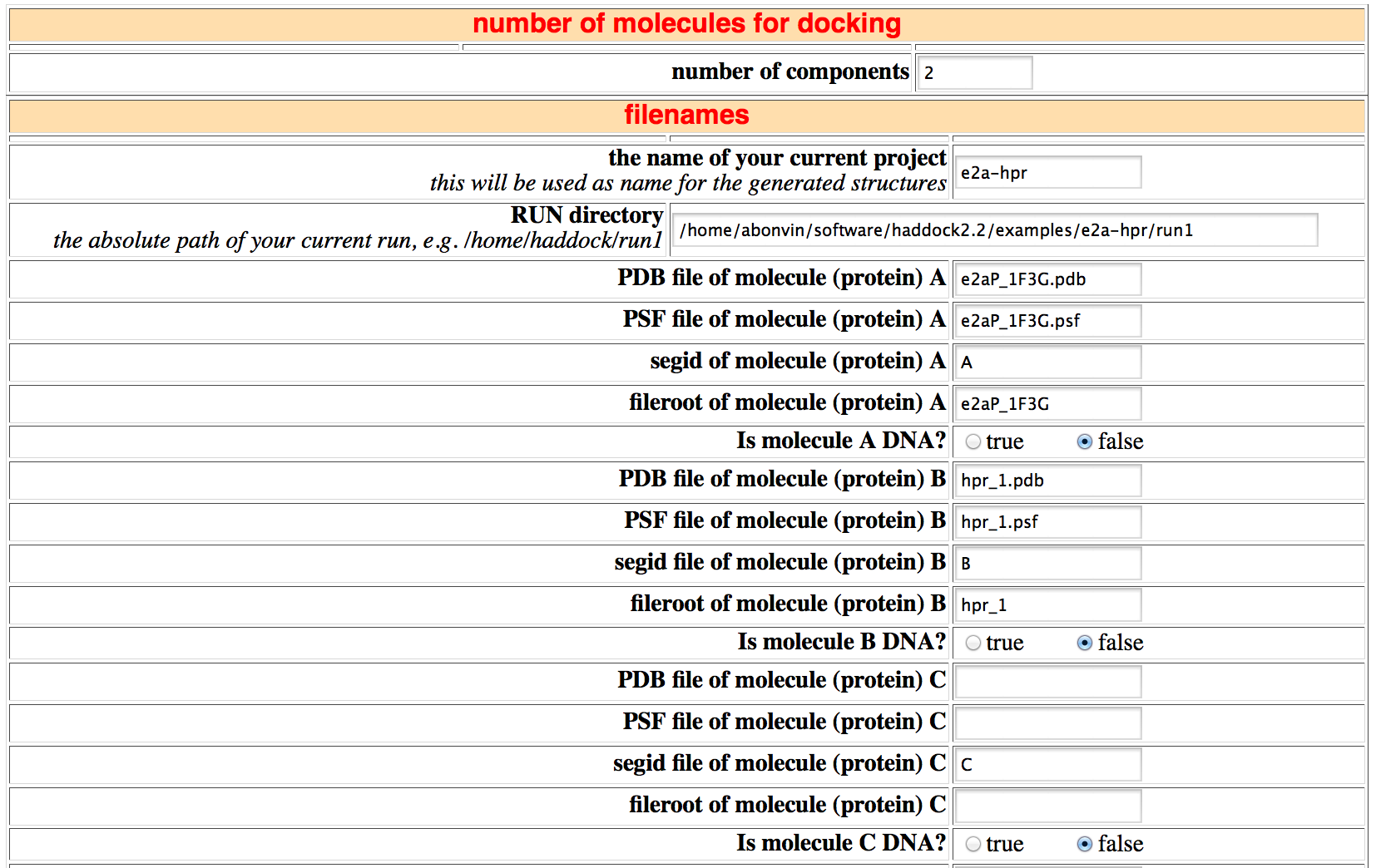
This section consist of all the files that will be used for the docking. If the new.html file has been set up properly, most fields will be set correctly. The only thing you might want to change is the name of the current project which is used as as rootname for all files.
If one of the molecules is DNA (and not RNA!), set the DNA flag to true. This is needed since the building blocks in the DNA/RNA topology file correspond to RNA. When DNA is set to true, a patch will be applied to remove 2' hydroxyl groups.
Also check that the HADDOCK directory, defining the path to the HADDOCK programs, is correct.
-
Note 1: Do not change the name of the input PDB file otherwise it will not be found by HADDOCK (this
file corresponds to the one you previously defined in new.html.
Note 2: Do not use similar names for the various molecules and the name of the current project.
In that section there is also a paramater that defines if non-polar protons should be kept or not:
{* Remove non-polar hydrogens? *}
{+ choice: true false +}
{===>} delenph=true;
By default non-polar protons are deleted to speed-up the calculations. They are however accounted for in the heavy atoms parameters since the force field used (OPLS) is a united atom force field.
-
Important: In case you are defining distance restraints involving non-polar protons (e.g. NOE restraints), make sure to set delenph to false, otherwise your restraints will not be used! To make sure all your restraints are properly read, it is recommended to check one of the generated output file for a model (e.g. from the rigid body docking) and search for error messages related to the NOE restraints (NOESET-INFO).
3. Definition of the protonation state of histidines
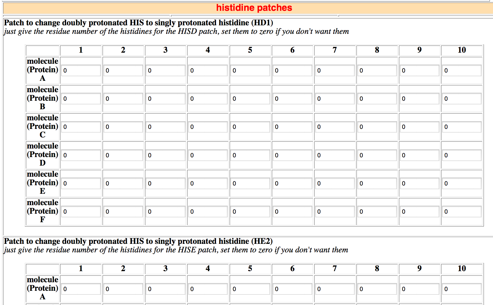
By default, all histidines are protonated and thus carry a net positive charge. In this section you can specify the protonation state of histidines for each protein. A neutral histidine can exist in two forms:
- HISD: the imino proton is attached to the ND1 nitrogen
- HISE: the imino proton is attached to the NE2 nitrogen
4. Definition of the semi-flexible interface
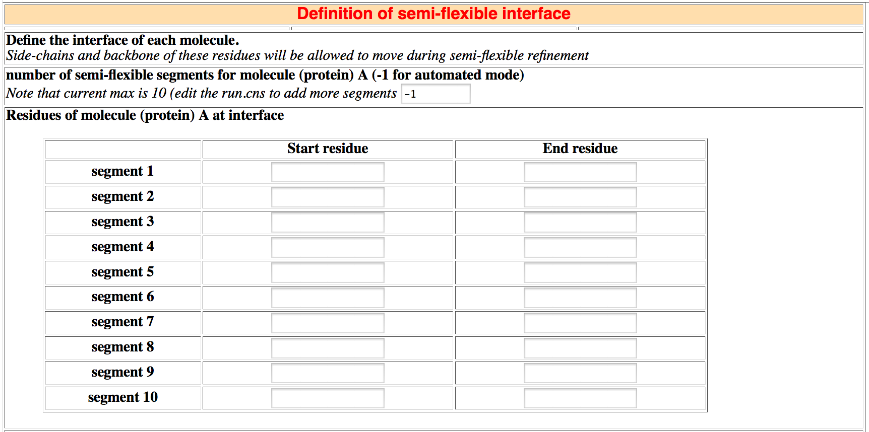
HADDOCK performs a semi-flexible simulated annealing (SA). Here you have to define the residues that will be allowed to move during the SA.
In HADDOCK 2.X, you have two options:
Manual definition of the semi-flexible segments
Usually we define as flexible residues all active and passive residues +/- 2 sequential residues.
For each molecule, enter the number of flexible segments and then the starting and ending residue of each segment.
- Note that the maximum number of segments is 10 for each
molecule. To add more segments, edit the run.cns file (See the FAQ section).
Automated mode (default)
HADDOCK 2.X offers the possibility to automatically define the semi-flexible residues. This is done automatically for each structure by selecting all residues that make intermolecular contacts within a 5A cutoff. You can change this cutoff value by editing the flexauto.cns CNS script in the protocols directory.
To turn on the automated mode, the number of segments should be a negative number (default: -1). Since HADDOCK2.X also allows to randomly define ambiguous interaction restraints from the defined semi-flexible segments (see the distance restraints section below), this number could also be larger (e.g. -3 to define three segments from which to randomly define AIRs. As long as the number is negative, the semi-flexible residues will be defined automatically.
5. Definition of fully flexible segments
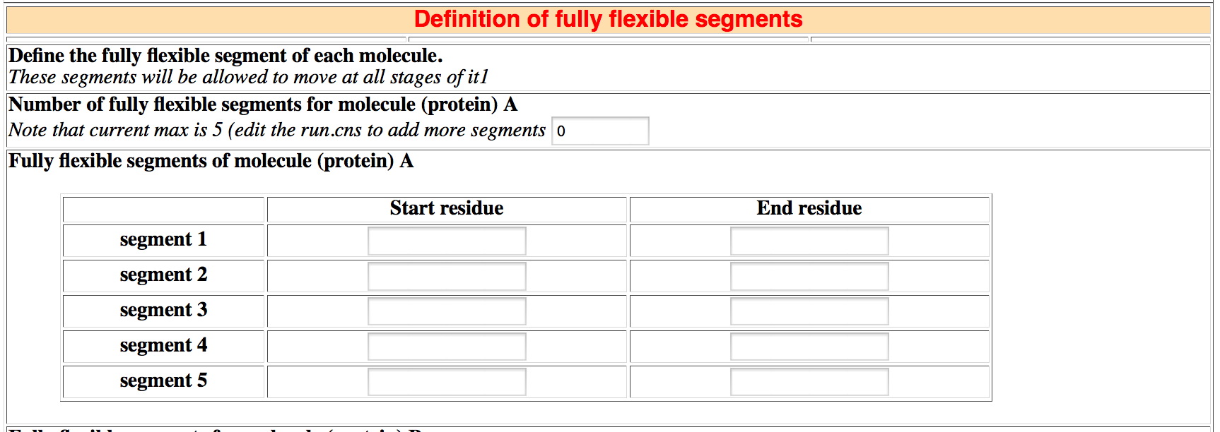
HADDOCK allows the definition of fully flexible segments for each molecule. These will be fully flexible throughout the entire docking protocol except for the rigid body minimization (see the docking section).
For each molecule, enter the number of fully flexible segments and then the starting and ending residue of each segment.
- Note that the maximum number of fully flexible segments
is 5 for each molecule. To add more segments, edit the run.cns file
(See the FAQ section)..
6. Symmetry restraints
This section allows to define two types of restraints to enforce symmetry either within or between molecules:
- non-crystallographic symmetry restraints (NCS)
- C2, C3, S3, C4 and C5 symmetry restraints
Non-crystallographic symmetry restraints (NCS)
The NCS option imposes non-crystallographic symmetry restraints: it enforces that two molecules, a fraction thereof or even two sub-domains within the same molecule should be identical without defining any symmetry operation between them.
HADDOCK 2.X allows to define up to five pairs for which NCS restraints will be applied. The syntax is fully flexible since start and end residues can be defined together with the molecule SEGID. In that way both intermolecular and intra-molecular NCS restraints can be defined.
-
Note: Since all atoms will be used for the definition of NCS restraints, it is important the NCS
pairs contain exactly the same number of atoms.
C2, C3, S3, C4 and C5 symmetry restraints

HADDOCK 2.X offers the possibility to define multiple symmetry relationships within or in between molecules. This is done by using symmetry distance restraints (Nilges 1993). Symmetry distance restraints are a special class in CNS: for each restraint two distances are specified which are required to remain equal during the calculations, irrespective of the actual distance. They can be defined in CNS as:
noe
    class symm
    assign (resid 1 and name CA  and segid A)
            (resid 50 and name CA  and segid B) 0 0 0
    assign (resid 1 and name CA  and segid B)
            (resid 50 and name CA  and segid A) 0 0 0
end
noe
   potential  symm symmetry
end
By defining multiple pairs of distances between the CA atoms of two chains, C2 symmetry can be enforced.
This can be easily extended to higher symmetries by defining multiple pairs of symmetry restraints:
- for C3, one can define three pairs of distances that should be equal:
- C5 symmetry can be enforced by defining five pairs:
- A-B = B-C, B-C = C-A and C-A = A-B
- A-C = A-D, B-D = B-E, C-E = C-A, D-A = D-B and E-B = E-C
-
Note: By combining multiple symmetry restraints is is possible to enforce other symmetries.
For example D2 symmetry in a tetramer can be defined by imposing six C2 symmetry pairs:
A-B, B-C, C-D, D-A, A-C and B-D.
7. Distance restraints
Ambiguous (AIRs) and unambigous distance restraints
Ambiguous (AIRs) and unambigous distance restraints specified in new.html will always be read. In this section, however, you can specify the stage of the docking protocol at which a given type of distance restraint will be used for the first and last time:
- 0: rigid body EM (it0)
- 1: semi-flexible simulated annealing (SA) (it1)
- 2: explicit solvent refinement (water)
- hot: high temperature rigid body dynamics
- cool1: first rigid body slow cooling SA
- cool2: second slow cooling SA with flexible side-chains at interface
- cool3: third slow cooling SA with flexible side-chains and backbone at interface
Random removal of AIRs
HADDOCK offer the possibility to randomly remove a fraction of the AIRs (only active on the ambiguous interaction restraints defined in ambig.tbl for each docking trial. This option is particularly useful when the accuracy of the AIRs is questionable since by random removal bad restraints could be discarded, allowing for better docking solutions.
To enable random removal of restraints, set noecv to true and define the number of sets into which the AIRs will be partitioned; one set will be randomly discarded. By setting for example the number of partitions (npart) to 2, 50% of the AIRs will be discarded for each docking trial; for npart=4 25% of the AIRs will be randomly discarded.
Hydrogen bond restraints
Define here if you want to use hydrogen bond restraints. The restraint file should have been specified in new.html.
Random interaction restraints definition
Define here if you want to randomly define interaction restraints (AIRs) from solvent accessible residues. The sampling will be done from the defined semi-flexible segments. To sample the entire surface, define the entire sequence as semi-flexible and use the automated semi-flexible segment definition to limit the amount of flexibility to the interface region. For more details see the AIR restraints section of the online manual.
Random AIRs are only active during the rigid body stage of the docking protocol. For the semi-flexible refinement, one AIR will be automatically defined between all residues within 5A from another molecule. No AIRs will be active during the final explicit solvent refinement.
-
Note1: Random AIRs are exclusive with ambiguous, unambigous and hydrogen bond restraints defined in
new.html. They can however be combined with surface and center of mass restraints (see below).
Define here if you want to use center of mass restraints and specify the corresponding force constant. Can be useful in combination with random interaction restraints definition (see above).
Surface contact restraints
Define here if you want to use surface contact restraints and specify the corresponding force constant. This can be useful in combination with random interaction restraints definition (see above).
Automatic weighting of distance restraints
Also available is an option to automatically adjust the force constant of the distance restraints (sum of distance and AIRs) to balance the distance restraint energy with the sum of the force field energy terms (bonds, angles, dihedrals, electrostatic and van der Waals) such as the ratio of force field energy versus distance restraint energy is equal to 2. For this you need to specify the number of distance and AIR restraints. The automatic scaling option will not appear when editing the run.cns file in a web browser. You will have to edit the file manually for this.
- Note: This option has not been thoroughly tested. An upper
limit of 5000 is set for distance restraining force constant. For
more details have a look at the set_noe_scale.cns script in
the protocols directory.
8. Radius of gyration restraint
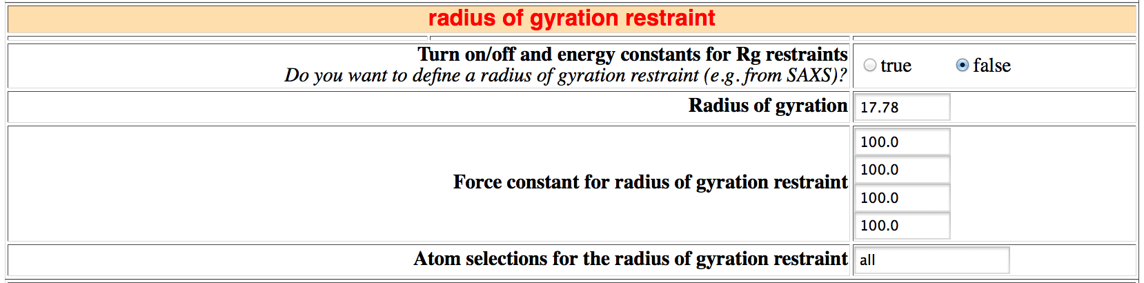
A radius of gyration distance restraint can be turned on here. It will be active throughout the entire protocol, but can be effectively turned off by setting the force constant for a given stage to 0. The radius of gyration should be entered in angstrom. By default it is applied to the entire system, but can be restricted to part of the system using standard CNS atom selections.
For example to limit it to chains B and C define:
- (segid B or segid C)
9. DNA/RNA restraints
Define here if you want to use DNA/RNA restraints. To use such restraints, edit the dna-rna-restraints.cns file provided in the protocols directory (you can use the same mechanism for that as for editing the run.cns parameter file from the project setup menu of HADDOCK), adapt it to your particular case, and place it in the data/sequence directory. This file allows you to define base-pair, backbone dihedral angle and sugar pucker restraints.
10. Dihedrals
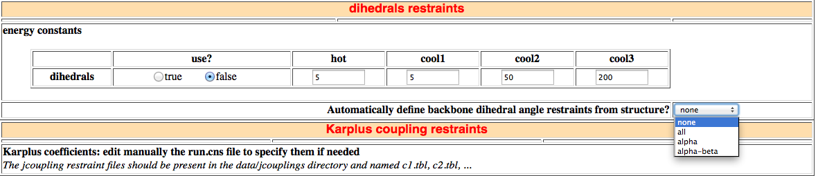
If dihedral angle restraints have been defined in the new.html file, turn the flag "use" to true and specify the force constants for the various stages of the semi-flexible simulated annealing (for water the value of cool3 will be used).
HADDOCK2.2 offer a new option to automatically dihedral angle restraints from the input structures. By default it is turned off, but you can specify to define dihedral angle restraints for the entire backbone, alpha-helices only or alpha-helices and beta-sheets. The secondary structure elements are defined based on a simple phi/psi dihedral angle criterion.
11. Karplus coupling restraints
You can specify in this section the Karplus coefficients and force constants for J-coupling restraints. This should directly be edited in the run.cns and will not show up in a browser window.
12. Residual Dipolar couplings

If RDC data are available and have been defined in the new.html file, you can define them in this section. Five classes are supported. For each class you can specify the type of function:
- SANI: direct refinement against the dipolar couplings (a tensor will be
included in the structures calculations)
- VANGLE: refinement using intervector projection angle restraints
(Meiler et al. J. Biomol. NMR 17, 185 (2000))
You can specify the first and last stage at which the various RDCs will be used.
- 0: rigid body EM (it0)
- 1: semi-flexible simulated annealing (SA) (it1)
- 2: explicit solvent refinement (water)
For SANI Da (in Hz) and R (R=Dr/Da) should be specified. You should also specify the force constants for the various stages of the docking protocol:
- hot: high temperature rigid body dynamics
- cool1: first rigid body slow cooling SA
- cool2: second slow cooling SA with flexible side-chains at interface
- cool3: third slow cooling SA with flexible side-chains and backbone at interface
13. Pseudo contact shifts
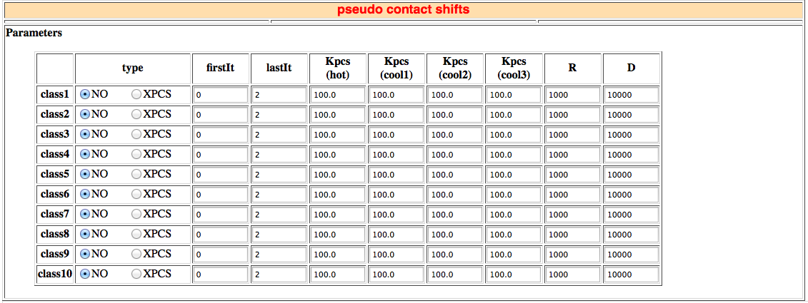
If pseudo contact shift data are available and have been defined in the new.html file, you can define them in this section. Ten classes are supported. For each class you can specify the first and last stage at which the various RDCs will be used.
- 0: rigid body EM (it0)
- 1: semi-flexible simulated annealing (SA) (it1)
- 2: explicit solvent refinement (water)
- hot: high temperature rigid body dynamics
- cool1: first rigid body slow cooling SA
- cool2: second slow cooling SA with flexible side-chains at interface
- cool3: third slow cooling SA with flexible side-chains and backbone at interface
For more information on using diffusion anisotropy as restraints for docking see also the PCS restraintssection of the online HADDOCK manual. Refer to the following publication for details of the implementation in HADDOCK:
- C. Schmitz and A.M.J.J. Bonvin
Protein-Protein HADDocking using exclusively Pseudocontact Shifts.
J. Biomol. NMR, 50,, 263-266 (2011).
14. Diffusion anisotropy restraints
If diffusion anisotropy restraints (DANI) (from 15N relaxation measurements) are available and have been defined in the new.html file, you can define them in this section. Five classes are supported (e.g. for measurements at different fields).
You can specify the first and last stage at which the various DANI restraint sets will be used.
- 0: rigid body EM (it0)
- 1: semi-flexible simulated annealing (SA) (it1)
- 2: explicit solvent refinement (water)
- hot: high temperature rigid body dynamics
- cool1: first rigid body slow cooling SA
- cool2: second slow cooling SA with flexible side-chains at interface
- cool3: third slow cooling SA with flexible side-chains and backbone at interface
15. Topology and parameters files
In this section the topology, linkage and parameter files are specified for each molecule. The default values are for proteins using the improved parameters of Linge et al. 2003 and OPLSX non-bonded parameters.
For dna use instead the dna-rna-allatom.top, dna-rna-allatom.param and dna-rna.link files in the toppar directory.
Also provided in the toppar directory in this version of HADDOCK are topologies and parameters for heme groups. See for this the topallhdg.hemes and parallhdg.hemes files. An example of distance restraints to maintain non-covalently attached heme in place is given in metalcenter.tbl in the toppar directory.
topallhdg.hemes also contains a number of patches to covalently attach the heme group to CYS and HIS residues. These patches should be added manually to the generate_X.inp when needed (an example is provided but currently commented out; search for heme in the file). (These files were kindly provided by Gabriele Cavallaro, CERM Firenze).
Parameter and topology files for small ligands should be provided by the user and place in the toppar directory (see also the FAQ section of the online manual).
In this version of HADDOCK, ions should be automatically recognized provided their naming is consistent with what is defined in the ion.top topology file in the toppar directory. For the torsion angle dynamics part of the docking protocol (it1), a covalent bond will be automatically defined to the closest ligand atom (only for cations). This is done in the covalions.cns CNS script in the protocols directory; the following cations are currently defined: MG+2, CA+2, FE+2, FE+3, NI+2, CO+2, CO+3, CU+1, CU+2 and ZN+2. If your system contains other ions add them to the covalions.cns file (they should however be defined in ion.top).
16. Energy and interaction parameters
You can define in this section a number of parameters that control the electrostatic energy term during the docking process, that allow you to scale down the intermolecular interactions and sample 180 degrees rotated solutions.
Electrostatic treatment
The electrostatic energy term can be turned on or off for the first two stages of the docking, namely the rigid body minimization and the semi-flexible simulated annealing. Two implementations are now supported to describe the solvent implicitly:
- constant dielectric
- distance dependent dielectric
For the final stage, the explicit solvent refinement, a constant dielectric with an epsilon equal to one is used by default.
Scaling of intermolecular interactions
This section also allows you to specify scaling factors for the various stages of the docking:
- rigid body EM
- rigid body dynamic: high temperature and slow cooling SA rigid body dynamics
- second slow cooling SA with flexible side-chains at interface
- third slow cooling SA with flexible side-chains and backbone at interface
-
Note: It might be useful to scale down the intermolecular interactions during rigid-body
docking in cases where a ligand has to penetrate in a deep and (partly) buried pocket
of a protein. A value of 0.01 should already be sufficient for this.
Interaction matrix for non-bonded interactions
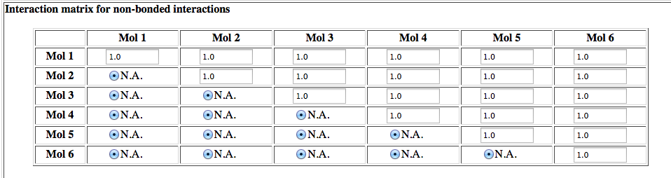
This is a new feature in HADDOCK2.2 which allows to scale down or turn off interactions between specific molecules. It is useful for example in the context of ensemble-averaged docking where the distance restraints should be averaged over multiple binding poses. This option has been applied for example in ensemble-averaged docking of a peptide using PRE-derived distance restaints. See:
-
E. Escobar-Cabrera, Okon, D.K.W. Lau, C.F. Dart, A.M.J.J. Bonvin and L.P. McIntosh
Characterizing the N- and C-terminal SUMO interacting motifs of the scaffold protein DAXX.
J. Biol. Chem., 286, 19816-19829 (2011).
17. Number of structures to dock
The docking process is performed in three distinct steps:
- rigid body minimization (it0)
- semi-flexible simulated annealing (it1)
- explicit solvent refinement (water)
Sampling of 180 degrees-rotated solutions
This is a new option in HADDOCK 2.X that allows sampling of 180 degrees-rotated solutions at both the rigid-body and semi-flexible docking stages. If turned on (default for rigid-body stage), for each model generated, a 180 degree rotated solution will be generated automatically by HADDOCK and either energy minimized (rigid-body) or submitted to the semi-flexible refinement protocol (it1). The rotation axis is automatically defined from the vector connecting the center of masses of the two interfaces, each interface being defined by all residues forming intermolecular contacts within 5A (this cutoff is defined in the rotation180.cns CNS script in the protocols directory.
Sampling of 180 degree rotated solutions in the rigid-body stage clearly improve the docking performance (unpublished data). If turned on during the semi-flexible refinement, both refined solutions will be written to disk, doubling the effective number of structures.
-
Note1: The sampling of 180 degree-rotated solutions in the semi-flexible refinement is not advised
since it might lead to unrealistic structures (e.g. with knots!). If used, carefully check the
resulting structures for artifacts.
-
Note2: If solvated docking is turned on, then the sampling of 180 degree-rotated
solutions will be automatically turned off during the calculations.
18. DOCKING protocol

Here you can define parameters for the rigid-body docking step (it0) if you want to:
- cross-dock all combinations in the ensembles of starting structures (should be turned off for example if you only want to perform water refinement of a preformed complex)
- randomize the starting orientations or not
- perform the rigid body minimization or not
- allow translation during the minimization (it can be useful to turn it off for docking highly flexible small molecules (see the docking section of the online manual)).
The next parameters govern the semi-flexible simulated annealing protocol. You can define the start and end temperatures and the number of integration steps for the various stages of the annealing protocol (see the docking section).
-
Note: If solvated docking is turned on, then the number of MD steps for
the rigid body stages of the semi-flexible refinement (high temperature rigid-body TAD and slow
cooling annealing) will automatically be set to 0 during calculations.
19. Solvated docking
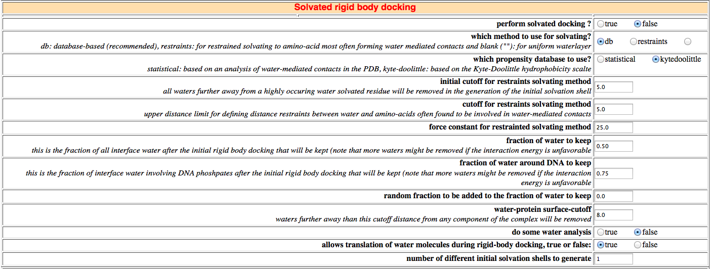
In this section you can turn on solvated docking. If turned on, the initial structures will first be solvated in a shell of TIP3P water (only water molecules within 5.5 A of the protein will be kept). The rigid-body docking will thus be performed from solvated proteins. Two methods for dealing with interfacial waters are implemented:
- database-based (db) (recommended upon restrained solvated docking (see below)): interfacial
water molecules will be removed in a biased Monte Carlo
process until a user-defined fraction of water remain. This process can make use of two different propensity scales:
- propensities of finding water-mediated contacts between amino-acid pairs defined from a statistical analysis of high-resolution
crystal structures. The water-mediated contact propensities can be found in the db_statistical.dat CNS
script in the protocols directory.
For details see:
- A.D.J. van Dijk and A.M.J.J. Bonvin.
"Solvated docking: introducing water
into the modelling of biomolecular complexes." Bioinformatics, 22 2340-2347 (2006).
- propensities of finding water-mediated contacts between amino-acid pairs defined from the Kyte-Doolittle hydrophobicity scale.
The corresponding water-mediated contact propensities can be found in the db_kyte-doolittle.dat CNS
script in the protocols directory.
For details see:- P.L. Kastritis, K.M. Visscher, A.D.J. van Dijk and A.M.J.J. Bonvin
Solvated docking using Kyte-Doolittle-based water propensities.
Proteins: Struc. Funct. & Bioinformatic, 81, 510-518 (2013).
An important parameter to be defined for database-solvated docking is the fraction of interfacial water to be kept after the Monte Carlo removal process. This is currently set to 50% based on our analysis of water-mediated contacts. New in HADDOCK2.2, this percentage can now be defined separately for nucleic acids (currently 75%). This is coming from the observation that nucleic acids show typically higher solvation. For details regarding nucleic acids solvated docking see:-
M. van Dijk, K. Visscher, P.L. Kastritis and A.M.J.J. Bonvin.
Solvated protein-DNA docking using HADDOCK.
J. Biomol. NMR, 56, 51-63 (2013).
Note that typically less than that (or even none) of the water molecules will be kept since an energy cut-off is applied after the Monte Carlo water removal step: all waters with unfavorable interaction energies (Evdw+Eelec>0) are removed. In some cases, this allows all interfacial waters to be removed at the end. The energy cutoff is defined in the db1.cns CNS script in the protocols directory.
- propensities of finding water-mediated contacts between amino-acid pairs defined from a statistical analysis of high-resolution
crystal structures. The water-mediated contact propensities can be found in the db_statistical.dat CNS
script in the protocols directory.
- restrained solvating (restraints): in this approach, water molecules are restrained to be at proximity
of amino-acids found to form the most water-mediated contacts (arg, asn, asp, gln, glu, his, lys, pro,
ser, thr and tyr). This is done by defining ambiguous distance restraints between each water and highly
solvated amino-acids on both side on an interface. Note that this method has not been
thoroughly tested.
If restrained solvating is chosen, three additional parameters should be set:
- initial distance cutoff: all water molecules further away from a highly solvated amino-acid will be removed in the solvent shell generation step.
- initial distance cutoff: upper distance restraints for the definition of ambiguous water-amino-acid restraints.
- force constant for water-amino-acid distance restraints.
It is also possible to turn off water translation during rigid-body energy minimization if desired.
Finally, to increase sampling, it is possible to start the docking from differently solvated molecules. The number of initial solvation shells can be define here. If more than 1 is defined, the protein will be randomly rotated and a new solvation shell will be generated.
20. Final explicit solvent refinement

In this section you can define if the final explicit solvent refinement should be performed (recommended since it does improve the docking solutions) and on how many structures. Two solvent models are currently supported: water and DMSO. DMSO is a fair mimic for a membrane environment.
You can also specify here the number of MD integration steps for the heating, sampling and cooling phases of the explicit solvent refinement.
You can also specify to keep the solvent, in which case an additional PDB file will be created in the structures/it1/water directory with a _h2o.pdb extension containing both your complex and the solvent molecules.
21. Scoring
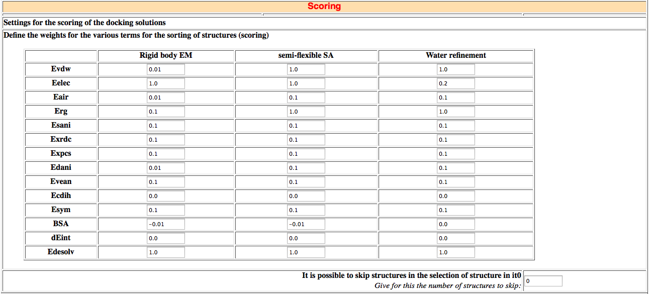
In this section you can define individual weigths for the various terms using in scoring. This can be done separately for the various docking stages (rigid body (it0), semi-flexible refinement (it1) and explicit solvent refinement(water)). You can also define the number of structures to analyze after the simulated annealing and explicit solvent refinement.
This version of HADDOCK offers a fully flexible scoring scheme since the weight of the various energy terms can be defined separately for each phase of the docking. The scoring is performed according to the weighted sum (HADDOCK score) of the following terms:
- Evdw: van der Waals energy
- Eelec: electrostatic energy
- Eair: distance restraints energy (only unambiguous and AIR (ambig) restraints)
- Erg: radius of gyration restraint energy
- Esani: direct RDC restraint energy
- Evean: intervector projection angle restraints energy
- Epcs: pseudo contact shift restraint energy
- Edani: diffusion anisotropy energy
- Ecdih: dihedral angle restraints energy
- Esym: symmetry restraints energy (NCS and C2/C3/C5 terms)
- BSA: buried surface area
- dEint: binding energy (Etotal complex - Sum[Etotal components] )
- Edesol: desolvation energy calculated using the empirical atomic solvation parameters from Fernandez-Recio et al. JMB 335:843 (2004)
-
Note 1: The vdw and elec energy terms can be negative indicating favorable interactions.
Note 2: While smaller energy terms indicate improvement, a larger buried surface area should indicate a better interface. It is therefore recommended to use a negative weight for the BSA term (if included) to favor larger interfaces.
Note 3: If you modify the treatment of electrostatics during docking you should probably redefine the electrostatic weights for scoring of it0 and it1 structures since these have been optimized for the current default settings.
The default scoring function settings of HADDOCK are for protein-protein complexes and use the following weights:
     HADDOCKscore-it0   = 0.01 Evdw + 1.0 Eelec + 1.0 Edesol + 0.01 Eair - 0.01 BSA

     HADDOCKscore-it1   =  1.0 Evdw + 1.0 Eelec + 1.0 Edesol +  0.1 Eair - 0.01 BSA

     HADDOCKscore-water =  1.0 Evdw + 0.2 Eelec + 1.0 Edesol +  0.1 Eair
-
Note: Additional terms are used if other types of experimental restraints are used. Refer to run.cns for their default settings
Note: For protein-ligand (small molecule) docking we recommend to change the weight of Evdw(it0) to 1.0 and Eelec(water) to 0.1.
Note: For protein-nucleic acids docking we recommend to set the Edesol weight to 0 for all stages
In this section, you can also define a "skipping" parameter that allows you to sample more solutions from the rigid body EM docking (it0). If the value x of this skip parameter is larger than 0 then every (x+1)th structure from it0 starting from the first structure will be further refined in the semi-flexible simulated annealing.
For example, if skip=1 and 200 structures should be refined in the semi-flexible simulated annealing, structures 1,3,5,7,... and 399 from the best 400 of it0 will be selected and written to the file.nam, file.list and file.cns files in the structures/it0 directory. Three additional files (file.nam_all, file.list_all and file.cns_all) containing the original sorting of all structures will be created.
22. Analysis and clustering
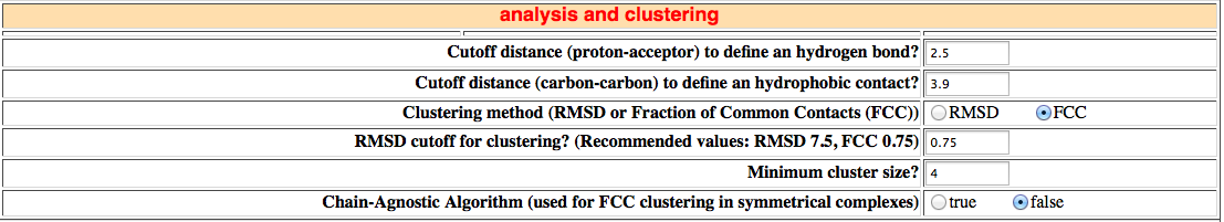
When performing the analysis, HADDOCK will check intermolecular hydrogen bonds and intermolecular hydrophobic contacts.
Here you can define the cut-off distances in Angstrom to define a hydrogen bond and a hydrophobic contact. Note that the hydrogen bond detection is only based on a distance criterion. For a more detailed analysis we recommend to use LIGPLOT (see software links.
At the end of the calculation, the solutions are clustered. Two options for clustering are offered:
- RMSD-based clustering using the tools/cluster_struc program (a small C++ program that needs to be compiled during installation). cluster_struc reads the output of the rmsd.inp CNS analysis script that generates the pairwise rmsd matrix over all structures analyzed and perform clustering. The RMSDs are calculated on the interface residues of the second molecule after fitting on the interface residues of the first molecule, what can be termed: interface-ligand-RMSD. The interface residues are automatically defined based on an analysis of all contacts found in all analysed models. Note that RMSD clustering might not be very discriminative in case of multibody docking.
- Fraction of native contacts (FCC) clustering using the tools/cluster_fcc.py python script. This option does not require a-priori fitting of the structures and is more robust for multibody docking.
For details see:
-
J.P.G.L.M. Rodrigues, M. Trellet, C. Schmitz, P.L. Kastritis, E. Karaca, A.S.J. Melquiond and A.M.J.J. Bonvin
Clustering biomolecular complexes by residue contacts similarity.
Proteins: Struc. Funct. & Bioinformatic, 80, 1810-1817 (2012).
The new FCC clustering offers the option to ignore chains when dealing with symmetrical oligomers. For example for a symmetrical trimer, this means that the ABC and ACB arrangements will cluster is the same cluster.
(For further details for manual analysis see Analysis for details).
23. Cleaning
Since HADDOCK does generate a lot of data and output files, we now built in a cleaning option. If turned on (default) all (except for the first structure of each stage) job, input and output files for the rigid-body, semi-flexible refinement and final explicit solvent refinement will be removed automatically upon completion. This saves a significant amount of space.
25. Parallels jobs
In this section you can define the way the structure calculation will be run, and the location of the CNS executable. Currently 10 nodes or queues can be specified.
If you are going to run HADDOCK on a multi-processor computer with for example 4 CPUs, the entries for the first row could be:
- queue command: csh (this will run the jobs in background on the local computer)
- cns executable: /software/bin/cns
- number of jobs: 4 (four jobs in parallel)
In Utrecht we are using two different batch queuing system (DQS and openPBS) that distribute the jobs on various linux clusters. Our entry for this setup is:
- queue command: ssub linux (ssub is a wrapper script for submitting to the batch queuing system and linux is the queue destination)
- cns executable: /software/bin/cns
- number of jobs: 10 (10 jobs in parallel)
Other ways of distributing jobs over a cluster are addressed in the FAQ section of the manual.