

Tutorial metadynamics / HADDOCK for ligand-protein docking
This tutorial consists of the following sections:
- Introduction
- System setup and MD simulations
- Analysis of the metadynamics simulation
- Cluster analysis of the trajectories
- Protein-ligand docking with HADDOCK
- Congratulations!
- References
Introduction
In this tutorial we will exploit enhanced sampling molecular dynamics, namely metadynamics [1] to improve the predictive power of molecular docking of small ligands to a protein target in the framework of an ensemble docking strategy [2]. Molecular docking is a widely used technique employed in Computer-Aided Drug Design [3] with the aim to drastically reduce the cost associated with the development of new drugs. A docking algorithm can be grossly split into two main tasks: i) the search for putative binding poses of the ligand onto the selected protein target(s); ii) the ranking of all generated poses, according to a given “scoring function” which should reproduce at best the free energy of binding of the complex. Docking is also the main computational method employed in virtual screening (VS) campaigns aiming to the identification of putative drug candidates in silico [3,4,5]. Clearly, a VS calculation should correctly rank native-like poses as the top ones, thus assigning them the highest score (i.e. the lowest binding free energy). Both the above tasks i) and ii) can be implemented in different ways, however, they are both subject to failures due to the intrinsic limitations of docking algorithms. Examples of these limitations include the reduced ability to sample conformations of the binding site in the presence of ligands and the difficulties associated to correctly account for entropic and de-solvation contributions in the scoring functions [3,4,6].
The sampling problem, which is the focus of the present tutorial, is a crucial issue in presence of significant structural changes of the protein receptor due to the interaction with ligands (mechanism known as induced fit [7], which induces at least changes in the orientation of side chains and more generally in the shape of the binding site. This is particularly relevant in the search for new drug candidates, for which experimental information regarding their complexes with the target protein is not always available. Several methods were developed in the past decades to deal with this issue, but a general and successful approach is still missing [6,8]. Among them, the ensemble-docking method was developed with the aim to account for the plasticity of the receptor by performing docking on multiple conformations obtained from experimental or computational means. The advantage of using multiple conformations is the increased probability to have in the pool of structures at least one featuring a bound-like conformation of the binding site, suitable to optimally dock the correct ligand(s). This approach was shown to improve the outcome of docking and VS calculations in many works published in the last years [2,3,5].
In this tutorial we will show how to further improve the predictive power of molecular docking in cases where even a long unbiased MD simulation is unable to generate bound-like conformations of a known difficult target. In particular, we consider the T4 phage beta-glucosyltransferase, which shows a large distortion at the binding site upon binding of its uridine diposphate substrate. Different conformations of the protein generated by enhanced-sampling MD simulations will be used in multiple docking runs with the HADDOCK2.2 webserver [9]. The results will be compared with those obtained using an ensemble of protein structures generated by a plain MD simulation of the apo system.
Throughout the tutorial, coloured text will be used to refer to questions or instructions.
This is a question prompt: try answering it! This is an instruction prompt: follow it! This is a VMD prompt: write this in the Tk Console! This is a Linux prompt: insert the commands in the terminal!
System setup and MD simulations
First, let’s create the directories needed for the tutorial. Open a terminal and type the following commands:
cd Tutorials/metaHADDOCK
mkdir -p Xray MD/plain/analysis MD/meta
Setting up the simulation system
First go to the Xray directory and download the pdb file of the apo-form of the T4 phage beta-glucosyltransferase (hereafter GLUCO) (PDB code: 1JEJ or use wget to download it directly from the terminal:
cd Xray
wget https://files.rcsb.org/download/1JEJ.pdb
What should you check before using a pdb file downloaded from the RCBS databank?
See solution:
It is customary to check the pdb files for possible issues when
running docking calculations. In particular, one should check for missing
residues (lines starting with the string “REMARK 465”) or missing atoms (lines
starting with the string “REMARK 470”).
Fortunately, our structure contain all the residues present in the aminoacid
sequence, as well as all the heavy atoms. For the sake of simplifying the
subsequent analysis, we will generate a “clean” pdb file without
crystallographic waters named apo_GLUCO.pdb and containing only the protein;
you can use your favorite text editor or
VMD1.9.3 from the terminal:
Once we have the structure of our protein target, we can generate the files needed to run the MD simulations. In this case, we are going to use GROMACS2016 [10] and so we need the topology file (top extension) containing information about atom types, bonded and non-bonded interactions, etc., and the initial structure file in the native format of GROMACS2016 (gro extension). A typical simulation flowchart for GROMACS2016 is reported in the official GROMACS manual
GROMACS was installed in the directory /opt/gromacs-2016-mpi-plumed.
To use the commands provided with this package, type the following command in your
terminal:
source /opt/gromacs-2016-mpi-plumed/bin/GMXRC
We will use the pdb2gmx tool to generate the topology and the initial
structure of the protein (gmx_mpi help commands prints a list of available
commands). Go to the MD directory and type:
cd ../MD
gmx_mpi pdb2gmx -f ../Xray/apo_GLUCO.pdb -o apo_GLUCO.gro -p apo_GLUCO.top -ignh
You can generate the topology according to a series of different force-fields, including the AMBER, OPLS, CHARMM, and obviously the GROMOS96 families. The following list of force-fields pops up when running the command above:
We will choose here the GROMOS96 54a7 force-field (option 14). Then, another screen will pop up:
Select option 3, as in our case we removed previously all crystallographic water molecules from the structure. In the output you will see a lot of information and warnings, but one important point regards the total charge, amounting to 6e:
For the following steps you’ll need some input files and pre-calculated data, which can be found in the directory: ../tutorial_files
Plain MD simulations in explicit solvent
We are going to run a MD simulation in explicit water using periodic boundary
conditions for the efficient treatment of electrostatic interactions [11]. We
first need to use the command editconf which will set the dimensions of the
box (and center the protein therein) for periodic boundary simulations with
explicit water. A triclinic box will be generated (option -bt), and the minimum
distance between the solute and the box will be set to 1.2 nm (option -d). To do
so, from your current position, type:
cd ../MD/plain
gmx_mpi editconf -f ../apo_GLUCO.gro -o apo-box.gro -bt triclinic -d 1.2
Next, we fill the box containing our protein with water molecules, and save
the corresponding structure and topology files. We will first copy the protein
topology file apo_GLUCO.top into apo-solv.top in order to use the last
file for the remaining steps and to keep the apo_GLUCO.top as a backup file.
cp ../apo_GLUCO.top apo-solv.top
Now, run the solvate command (we will choose the single point charge SPC
water model specified by the file spc216.gro) by typing:
gmx_mpi solvate -cp apo-box.gro -cs spc216.gro -o apo-solv-init.gro -p apo-solv.top
You can now check the topology file with your preferred text editor (e.g. vim apo-solv.top),
and, if not present, manually include the parameters of the water model in the topology file
by adding the following lines at the end of the file, before the entry [ system ]:
; Include water topology
#include "gromos54a7.ff/spc.itp"
We are now ready to generate the GROMACS input file (tpr extension), a
binary file containing all the information needed to perform the requested
calculations on the system of interest. This is done with the grompp
command, which needs both the structure and the topology files and also an
input file (mdp extension) containing the directives to run the simulation
(such as simulation type, pressure and temperature control flags, treatment
of long-range interaction flags, flags related to the information to be
printed and so on). The file em-pbc.mdp (available in the folder
tutorial_files/apoMD) sets the typical parameters needed to run a
structural relaxation of the system, which allows to (partially) remove the
steric hindrance due to clashing contacts between atoms of the protein
and/or solvent.
Copy the mdp file
cp ../../tutorial_files/apoMD/em-pbc.mdp .
and type the following command to generate the tpr file needed for the relaxation:
gmx_mpi grompp -f em-pbc.mdp -c apo-solv-init.gro -o em-pbc.tpr -p apo-solv.top
The tool grompp checks on the fly the values given to the parameters present in the mdp file, and generates possible notes and warnings. By default, the program fails when some warnings are generated, but the user can change this behavior by setting the “-maxwarn” flag to values larger than 0 (clearly after ensuring that all the warnings raised are “safe”).
You might remember at this point that the protein has a positive charge of
6e. To neutralize this charge, we can add counterions using the genion
command as follows (we report the more general command line to add both
positively and negatively charged ions, K+ and Cl- in this case):
gmx_mpi genion -s em-pbc.tpr -p apo-solv.top -o apo-solv-init.gro -pname K -nname CL -nn 6 -np 0
The following output will appear, prompting to select the group of solvent molecules for ions substitution. Six molecules of the selected group will be replaced by chlorine ions.
In this case, we see that there are three identical groups of molecules, 11
to 13, which identify waters. Type one of them in the console, e.g. 13. Note
that, as in the case of the solvate command, also with genion you might need
to edit a posteriori the apo-solv.top file by adding the following lines before
the entry [ system ]:
; Include ions
#include "gromos54a7.ff/ions.itp"
Run again the grompp command to generate the tpr file including ions:
gmx_mpi grompp -f em-pbc.mdp -c apo-solv-init.gro -o em-pbc.tpr -p apo-solv.top
We can now generate the ndx file, an index file containing groups of molecules and which can be customized according to the user needs. In the following we will only generate the file without changing anything with respect to the default:
echo quit | gmx_mpi make_ndx -f em-pbc.tpr -o apo-solv.ndx
You could have a look to this file with your preferred text editor. It
consists of entries starting with [ namegroup ], followed by lines
reporting the serial numbers of atoms within that group.
Now we are ready to perform the structural relaxation of our system with the
mdrun engine of GROMACS:
nohup gmx_mpi mdrun -v -deffnm em-pbc &
Wait a few seconds and check the output file em-pbc.log to understand if your run was successful.
The next step after structural relaxation is to perform a MD simulation
slowly heating the system up to the desired temperature. To save time here
we will set the temperature to 300 K quite abruptly. The file equil-pbc.mdp
(available in the folder tutorial_files/apoMD) contains the directives on
how to perform the MD simulation with explicit water and under periodic
boundary conditions.
Generate now the input file (tpr extension) needed to run the actual simulation:
Now you can start the simulation by typing the following command:
nohup gmx_mpi mdrun -deffnm equil-pbc &
Let the simulation go or kill the job (kill -9 <PID>; when needed, you could use pre-calculated data).
Metadynamics simulations
We are going to perform metadynamics simulations using GROMACS 2016.5 and PLUMED2.3.5, a plugin facilitating the implementation of different kinds of enhanced sampling techniques (and not only) in several simulation packages, using the same syntax independently of the specific engine used. Briefly, metadynamics is an enhanced-sampling technique, developed by Laio and Parrinello about 15 years ago [1]. It enforces systems to escape free energy minima by means of a history-dependent fictitious potential. The system is thus forced to explore conformations associated to other (meta)stable basins and/or free energy barriers. This is achieved by defining a set of collective variables (CVs, e.g. a distance, an angle, a dihedral angle and the number of contacts between two groups of atoms) which identify the relevant motions to be enhanced in order to steer the sampling of otherwise unreachable conformations. The exploration of the CVs phase space (which “drags” the system towards atomic conformations otherwise rarely visited) is forced through the deposition of “hills”, namely Gaussian-like potentials, added every nG steps of the simulation to the CVs space at the point corresponding to the system’s state. These Gaussian hills will generate a repulsive force which is transmitted to the real atoms of the system thus enhancing the conformational sampling. Clearly, a good CV should be associated with a “slow” motion of the system (in absence of bias), so that its value at conformations associated with different free energy basins will differ too. The choice of the CVs is indeed crucial to the success of a metadynamics simulation and some rules of thumbs to guide the choice of the height, width and deposition time have been outlined by Laio et al. [12]. It was shown that under proper conditions, metadynamics generates, in the CVs space, a free energy landscape representing an unbiased estimate of the underlying free energy [13]. Since its introduction, many flavors of metadynamics were introduced [14] whose description is out of the scope of this tutorial. Here we will use the so-called “Well Tempered Metadynamics” [15], that represents an improvement over the original algorithm thanks to the possibility of controlling the regions of the free energy surface that are physically meaningful to explore.
Often a single CV is not sufficient to catch the relevant slow modes involved in the structural transition of interest. Indeed, all the CV-based methods often exploit the use of multiple variables, which ideally should be orthogonal to each other to enhance the sampling along independent directions of the CV space. A clever method to enhance sampling across a virtually unlimited number of CVs is the so-called bias-exchange metadynamics [16]. In bias-exchange metadynamics many simulations of the system at the same temperature are performed, biasing each replica with a time-dependent potential added to a different CV. Exchanges between the bias potentials in the different variables are periodically allowed according to a replica exchange scheme. Due to the efficaciously multidimensional nature of the bias, the method allows to explore complex free energy landscapes with high efficiency. In order to perform a metadynamics simulation, we need first to define our CVs. Here we will enhance the conformational sampling locally at the binding site (BS) of the apo-form of GLUCO, by biasing both the radius of gyration of the BS as well as the intramolecular contacts among the residues lining that site.
BS definition and CVs set-up
To define the BS, we exploit the crystallographic structure of the GLUCO-UDP complex. Namely we define the BS as the site lined by all residues having at least one atom within 4 Å from UDP. From the RCBS pdb databank download PDB ID: 1JG6 in the Xray directory, or use wget to download it from the terminal:
wget https://files.rcsb.org/download/1JG6.pdb
We will now generate a “clean” pdb file holo_GLUCO.pdb containing only the
protein and the UDP molecule, using VMD from the terminal (here you must
specify the resname of the uridine diphosphate substrate, UDP):
In this case we care going to define our BS on the hydrogenated holo structure (which you can obtain with software such as BABEL). Copy the hydrogenated holo we have already prepared for you from the tutorial_files folder:
cp ../tutorial_files/apoMD/holo_GLUCO.pdb .
Open the file with VMD again, and get the resid numbers of all aminoacids lining the BS:
You will see a VMD Main window, as well as a Display and a Graphics representation window.
Go to “Extension”
Select “Tk Console”, as shown in Figure 1
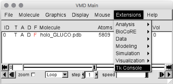
Figure 1: VMD Main screen, showing how to open the Tk Console
Within the Tk Console, type the following:
You will get the following list of residue numbers:
18 188 189 191 195 213 214 237 238 240 243 261 268 269 272
And a similar list containing the atom numbers (serials) of BP’s residues.
As a further example, suppose you are now interested only in the residues which are not hydrophobic (this choice could be justified by the nature of the UDP substrate, bearing a -3e charge). This can be easily done as follows:
You will get the following list of residue numbers:
187 188 189 191 195 214 237 261 269 272
Another useful parameter that we can extract from the experimental structure of the holo protein is the Radius of Gyration (RoG) of the BP, which indicates how compact (i.e. open or closed) is the binding pocket. Larger values of the RoG should correspond to more open conformations of the BP. Since the binding of a small ligand to the BP of a protein often causes a partial collapse of the pocket, we expect the RoG of the holo to be smaller than that of the apo protein. We can calculate the value of the BP RoG in the experimental structure through VMD by typing the following command in the Tk Console:
You will get the value (in Å) corresponding to the RoG of the BP (take a note as we will need this value later). Now you can close VMD.
As you will see below, PLUMED [17] needs atomic serial numbers as input. Thus, to
perform the simulation, we should get the list of serial numbers defining
the BP. We thus load the apo protein ready to be simulated into VMD and use
the residue list obtained previously to print the list of serials defining
the BS. Go to the ../MD/plain directory and copy there the em-pbc.gro file from the tutorial_files folder. Now open it on VMD.
cd ../MD/plain
cp ../../tutorial_files/apoMD/em-pbc.gro .
vmd -dispdev none em-pbc.gro
Now, paste into the Tk console all the following commands:
Note that with the previous commands we also calculated the value of the RoG of the BP for the apo structure, as we will also need this value later. Keep in mind that if you extract the serial number from the apo_GLUCO.pdb file, you will obtain different serial numbers (and this can happen with other systems as well, if different residues/atoms were unresolved in the apo and holo structures), not corresponding to the binding pocket atoms in the system that you are going to simulate! You should always cross-check the serial list before running the simulation!
Now we should check if the selected CVs are reasonable, and in that case, we
need to set the parameters of the Gaussian hills that are going to be
deposited during the metadynamics simulation. These parameters are: the
height of the hills (h), their width (w), and deposition time TAU_G. In
particular, w will be chosen by analyzing the evolution of the CVs along the
unbiased MD simulation. However, we will first analyze the simulation in
terms of structural distortions from both the starting apo and holo
experimental structures. You can use a pre-calculated trajectory file
called: equil-pbc.trr and the corresponding gro file em-pbc.gro, both
available in the folder tutorial_files/apoMD. Type:
The main window of VMD should appear as in Figure 2:
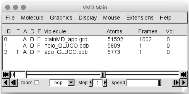
Figure 2: VMD Main screen, showing the data loaded. Note that, in your case, the
apo MD simulation will be called em-pbc.gro
Now, let’s calculate the Root Mean Square Deviation (RMSD) of the BS along the trajectory, both from the apo and holo experimental structures. In the VMD Main menu:
Go to the “Extensions” tab
Click and go to “Analysis”
then “RMSD Trajectory Tool”
You should see the menu displayed in Figure 3.
Let’s first estimate the RMSD from the holo experimental structure. We could
remove the apo experimental structure from the list of structures by
selecting the last line (corresponding to ID 2) and pressing Erase
Selected, after making sure the button Selected is marked.
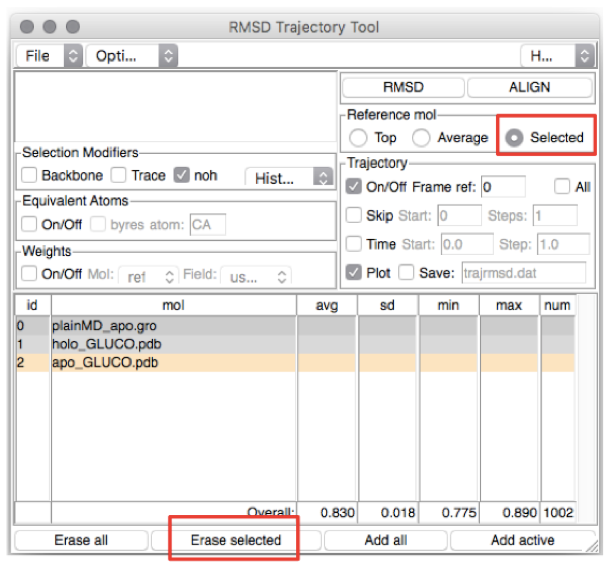
Figure 3: The VMD RMSD Trajectory Tool screen
In the top-left box type the residues you want to (align and) calculate the
RMSD of (in this case, the residues lining the BS). The list of residues is
found in the file BS_resid_numbers.dat in the Xray folder. Alternatively,
you can find them in the top-left red box in Figure 4. Now click on the line
corresponding to holo_GLUCO.pdb (ID 1) and tick Selected in the “Reference
mol” box (see Figure 4). Click on the ALIGN button (top-right red box in
Figure 4).
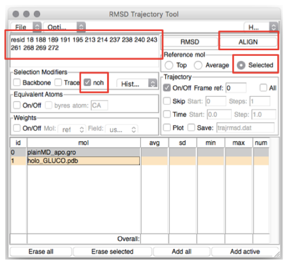
Figure 4: How to calculate the RMSD along a trajectory using VMD
Wait for a few seconds until the BS conformations sampled along the MD
trajectory are aligned to the BS of the reference structure, then select
Plot in the Trajectory box, and finally click the RMSD button in the
upright panel. You should obtain a plot which looks like the one in Figure 5:
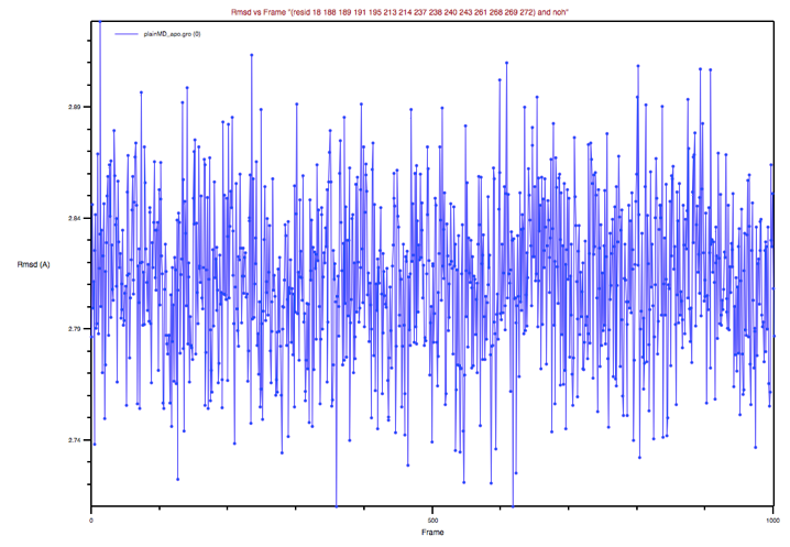
Figure 5: BP’s RMSD of the apo MD trajectory with respect to the holo
X-ray structure
Could you comment on this plot?
Now repeat the procedure above to estimate the RMSD of the BS from the apo
experimental structure. Note that you could bring back the apo_GLUCO.pdb
file by clicking on the Add all button adjacent to the Erase Selected
button that we used previously. Then you could delete the holo_GLUCO.pdb
molecule from the list and proceed as above. You should obtain a graph like
that shown in Figure 6.
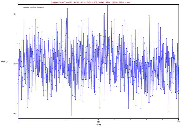
Figure 6: BP’s RMSD of the apo MD trajectory with respect to the apo
X-ray structure
Could you comment on this plot and its comparison to the previous one?
Now, let’s analyze the evolution of the CVs along the trajectory. To do this
we can use the tool driver of the PLUMED package. First, we need a text
file defining the CVs to be analyzed along the trajectory; driver will read
the trajectory and will print for each frame the values of the CVs selected
in the input file. From tutorial_files/Driver move the input file
plumed_driver.dat in the folder MD/plainMD/analysis, and type:
The output file COLVAR_driver lists the values of the CVs sampled along the
trajectory. (you can find a pre-calculated file in the
tutorial_files/Driver folder). To assess how much the CVs changed during
the unbiased MD simulation, plot their values with your preferred graph
viewer. Here we will use xmgrace.
Type the following commands:
These commands print the columns corresponding to the RoG and to the NCs
into two separate files and get rid of the first line which is not correctly
interpreted by xmgrace. For the sake of an easy comparison with the
experimental RoG values for the apo and holo X-ray structures let’s create a
simple text file containing these values. Open ref.dat in your current folder with your preferred
editor and type (the brackets < , > should not be included!)
Or, if needed, the file can be found in the tutorial_files/apoMD folder. Now we are ready to plot the CVs profiles. Type:
You will see a graph like that in Figure 7, showing the RoG of the BS of the structures sampled, together with the RoG for the experimental structures. A similar plot could be easily obtained also for the other CV chosen.
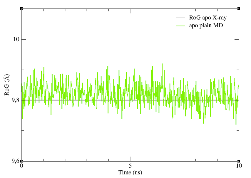
Figure 7: The RoG of the structures sampled during the apoMD simulation.
Despite it is preferable to perform these analyses on longer trajectories, you can see already from this graph that the CV we selected did not change significantly. Thus, they could be a good choice as CVs to enhance the sampling of different shapes and volumes of the BS.
Importantly, the analysis of the behavior of the CVs during an unbiased MD
simulation is useful to guide the choice of the width parameter of the
Gaussian-hills deposited during metadynamics. Indeed, it is customary to set
the value of w to be between 1/4 and 1/2 of the average fluctuations of a CV
during a short plain MD run [12,18],19]. Here, we calculate the standard
deviation of the CVs over 200 frames spaced 10 ps (thus 5000 MD steps) from
each other. You could calculate the standard deviation using your preferred
way, either by means of a graphics plot program such as xmgrace, or by
coding this into a script. Here, we will use the bash script av_std-sel-region-column.sh which can be found in the directory
tutorial_files/scripts to calculate the average and standard deviation of
our CVs. The script takes as input the name of the file containing the
values of the CVs, the column corresponding to the CV, the first and last
rows delimiting the size of the data, and the stride parameter to consider
one row every stride. As output, you will see on the terminal the average
and standard deviation of the CV corresponding to the column you chose. The
script can be used with the following command:
To perform the analysis described above, type:
The standard deviations of RoG and NCs will be used to set up the following metadynamics run.
Metadynamics simulations
To setup a metadynamics simulation with GROMACS and PLUMED we first need
three PLUMED files and an input file in the tpr format (which can be found
in the tutorial_files/plumed folder). As for the PLUMED files, they are:
- plumed-common.dat. It contains the definition of the CVs, in terms of the serial numbers of atoms to be biased within each of them, and additional information such as restraints, units, etc
- plumed.0.dat, plumed.1.dat. Each file contains the directive to read the plumed-common.dat file, as well as information on the bias to be applied to the related CV (such as its height and the frequency of deposition of the energy hills). In this case, we set the value of the bias factor to the default of 10. Instructions on names and writing-frequency of output files are also given.
More detailed information on how to run a metadynamics simulation can be found at the following webpages:
- General documentation on metadynamics with PLUMED
- Running metadynamics simulations with PLUMED
- Running Bias Exchange metadynamics simulations with PLUMED
Now go in the MD/meta folder created at the beginning of the tutorial and copy there:
i) the three plumed files just described, ii) the equil-pbc.tpr file used for the apo
simulation from the MD/plain folder. Now go to the MD/meta folder and create a tpr
file for each of the two replicas that we are going to run:
Open and read plumed-common.dat to understand clearly all the instructions. As you
can see the list of the atomic serial numbers is already encoded in the file. If not,
you should insert the list of serials previously extracted. Open now plumed.0.dat and
plumed.1.dat and insert the appropriate value of the sigma parameter where needed. You
should have calculated the w parameter (sigma) values in the previous section of this
tutorial by means of the av_std-sel-region-column.sh script.
You are now ready to run the simulation with the following command:
The flag “-replex” is used to specify th frequency of attempts to exchange the bias between the two replicas.
Wait for a few minutes and check the content of the directory. If the files COLVAR.X
and HILLS.X are being written (you can easily check with cat <filename> or wc -l <filename>) it means your simulation is running. As for the previous simulation, you
can use pre-calculated data to analyze the trajectory.
Analysis of the metadynamics simulation
Among the various files generated during a bias-exchange metadynamics simulation, the
most important ones are the files COLVAR.X (with X=0,1,…). These files report the
values of the CVs sampled by the system during the simulation, and thus allow assessing
if the sampling of the CVs is being enhanced or not. In this section, we will analyze
the MD trajectories mainly in terms of structural variation of the BS compared to the
experimental structure of the complex. We’ll start by plotting the profile of the RoG
as calculated along the MD trajectory. If our sampling strategy was successful, some
sampled structure should feature a RoG close to that of the experimental holo protein.
Copy the COLVAR.X and the ref_meta.dat files from the directory tutorial_files/plumed
to your working folder, then type the following commands:
Now type:
xmgrace -nxy ref_meta.dat RoG0.dat RoG1.dat
You should see a plot which looks like the one in Figure 8.
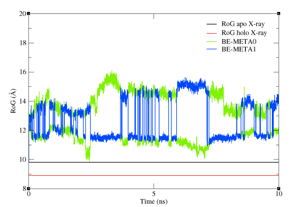
Figure 8: The RoG of the structures sampled during the BE-META simulation for both replicas, plotted against the
experimental value of apo structure’s RoG.
The simulation just performed and analyzed didn’t have any restraints on the values of the CVs. Although in principle they should sample all the conformational space available, in facts it could take a very long time to do so. To force sampling towards a predefined direction, you could insert some restraints on the CVs (a reader interested in how to set restraints during a metadynamics simulation with PLUMED can have a look here.
You can now compare the above graph with the following one (Figure 9), obtained from a metadynamics simulation with the same set-up as above, but featuring restraints on the RoG. Upper restraints were used on the RoG to force the system to explore conformations associated to smaller values than the initial one. By tuning the restraints according to your specific aims, you can force the sampling towards a given region of the conformational space.
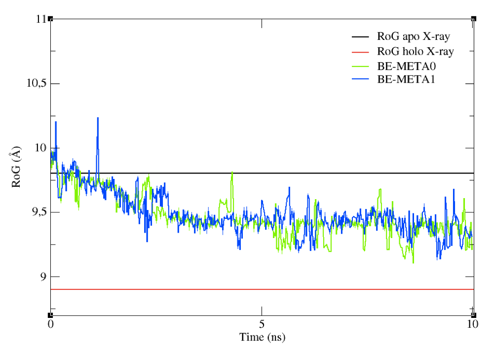
Figure 9: The effect on upper restraints of the RoG of the structures sampled.
Cluster analysis of the trajectories
To perform ensemble-docking runs a cluster analysis [20] must be performed so as to pick up a set of representative structures sampled by the protein (it would not be feasible to perform docking calculations on all of the structures sampled along MD simulations). Of course, while reducing the number of structures to consider, a good cluster analysis procedure should maximize the diversity of conformations sampled by the BP. In this way, if conformations prone to host the ligand were sampled during MD simulations, at least a representative for that “conformational mode” will be included in the pool of clusters that we are using for docking. Performing a successful cluster analysis, namely being able to actually include representatives of all the “conformational mode” remains a difficult task, and a lot of recipes have been proposed during the years [20]. Here we will perform a simple cluster analysis using the tool “cluster” within the GROMACS 2016 package with an RMSD cut-off of 2 angstroms on the BS.
We will perform the cluster analysis on both plain and metadynamics trajectories
(again, you could use pre-calculated clusters for the docking. Go to the directory
MD/plain and copy there the file apo-solv_withBS.ndx from
tutorial_files/cluster_analysis. To perform the cluster analysis only on the binding
pocket (and not, for example, on the whole protein), you need to edit the index file
(ndx extension) previously created, and insert there the serials of all residues
defining the BP. At the end of the apo-solv_withBS.ndx file, you should have
something like the following:
...
[ BS33 ]
172   174   175   176   177   178   179  1969  1971  1972  1973  1974  1976  1977  1978 [...] 2832  2835  2838  2839  2869  2871  2872  2873  2874  2875  2876  2877  2878
To run the cluster analysis type:
The following output will appear, asking you to select the region of the system that you want to consider:
Type 18 to select the binding site region.
Now, another output will be prompted, asking you what part of the protein we want to be written in the pdb file of each cluster. Of course, since we need to run docking calculations on those structures, we need the entire protein without water molecules. Type 1 and the cluster analysis will start.
This calculation can take up to several hours and for this reason we have already
pre-calculated 10 clusters coming from the apo plain MD and 10 clusters coming from the
BE-META. These simulations were from 10 to 100 times longer than the ones performed in
this tutorial (clearly, 10 ns are not enough to allow the binding pocket to reach the
RoG of the holo X-ray structure). You can find the clusters needed for the subsequent
docking calculations in ../../tutorial_files/cluster_analysis/clusters_ready/.
Protein-ligand docking with HADDOCK
Note that protein-ligand HADDOCKing typically requires fine-tuning a handful of parameters that requires the most advanced privilege on the web server. If you did not apply for the “guru” access level yet, it is time to apply for it via our registration portal. Alternatively, you can use the course credentials that were provided to you during the summer school to submit your docking runs. Please, use the pre-calculated runs to move on with the analysis section.
Setting up a new docking run targeting the identified binding pocket
We will now setup a docking run targeting specifically the identified binding pocket of the protein. For our targeted ligand docking protocol, we will first create two sets of restraints that we will use at different stages of the docking:
-
For the rigid-body docking, we will first define the entire binding pocket on the receptor as active and the ligand as active too. This will ensure that the ligand is properly drawn inside the binding pocket.
-
For the subsequent flexible refinement stages, we define the binding pocket only as passive and the ligand as active. This ensures that the ligand can explore the binding pocket.
In order to create those two restraint files, use the HADDOCK server tool to generate AIR restraints: https://alcazar.science.uu.nl/services/GenTBL/ (unfold the Residue selection menu):
18,188,189,191,195,213,214,237,238,240,243,261,267,269,272
1
Click on submit and save the resulting page, naming it GLUCO-UDP-act-act.tbl
Note: This works best with Firefox. Currently when using Chrome, saving as text writes the wrong info to file. In that case copy the content of the page and paste it in a text file.
Note: Avoid Safari for the time being - it is giving problems (we are working on it).
Now repeat the above steps, but this time entering the list of residues for the binding pocket into the passive residue list. Save the resulting restraint file as GLUCO-UDP-pass-act.tbl
Note: If needed, click on the links below to download two pre-generated distance restraints files:
The number of distance restraints defined in those file can be obtained by counting the number of times that an assign statement is found in the file, e.g.:
grep -i assign GLUCO-UDP-act-act.tbl | wc -l
Compare the two generated files: what are the differences? How many restraints are defined in each?
Note: A description of the restraints format can be found in Box 4 of our Nature Protocol 2010 server paper:
- S.J. de Vries, M. van Dijk and A.M.J.J. Bonvin. The HADDOCK web server for data-driven biomolecular docking. Nature Protocols, 5, 883-897 (2010). Download the final author version here.
We will now launch the docking run. For this we will make us of the guru interface of the HADDOCK web server:
https://alcazar.science.uu.nl/services/HADDOCK2.2/haddockserver-guru.html
Note: The blue bars on the server can be folded/unfolded by clicking on the arrow on the right
-
Step1: Define a name for your docking run, e.g. bemeta-ensemble or apoMD_ensemble.
-
Step2: Prepare the ensemble of 10 conformations that you will provide as starting structure for the protein.
HADDOCK accepts ensembles of conformations as starting files, provided all the coordinates are concatenated in one single PDB file and all the conformations contain EXACTLY the same atoms (same number, same names, same chain/segid, …). And easy way to prepare the “bemeta” and “apoMD” ensembles from the clusters files provided in the folder ../../tutorial_files/cluster_analysis/clusters_ready/ is to use pdb-tools.
- Step3: Input the protein PDB file. For this unfold the Molecule definition menu.
First molecule: where is the structure provided? -> “I am submitting it” Which chain to be used? -> All (for this particular case) PDB structure to submit -> Choose the proper ensemble file Segment ID to use during docking -> A
- Step 4. Input the ligand PDB file. For this unfold the Molecule definition menu.
Note: The coordinates of the ligand atoms must be submitted as HETATM and the residue number set to 1. You can download here the ligand coordinates if you want to proceed directly.
Since the structure of the ligand is directly obrained from the reference crystal structure of the complex, we can disable the flexibility of the ligand to enforce the bound conformation of the ligand in our models.
Second molecule: where is the structure provided? -> “I am submitting it”
Which chain to be used? -> All
PDB structure to submit -> Browse and select “ligand_clean.pdb”
Segment ID to use during docking -> B
Unfold the menu “Semi-flexible segments”
How are the flexible segments defined -> none
- Step 5: Input the restraint files for docking. For this unfold the Distance restraints menu
Instead of specifying active and passive residues, you can supply a HADDOCK restraints TBL file (ambiguous restraints) -> Upload here the GLUCO-UDP-act-act.tbl You can supply a HADDOCK restraints TBL file with restraints that will always be enforced (unambiguous restraints) -> Upload here the GLUCO-UDP-pass-act.tbl
Note: HADDOCK deletes by default all hydrogens except those bonded to a polar atom (N, O). In the case of protein-ligand docking however, we typically keep the non-polar hydrogens.
Remove non-polar hydrogens? -> FALSE (uncheck this option)
- Step 6: Change the clustering settings since we are dealing with a small molecule. For this unfold the Clustering parameter menu:
The default clustering method in the HADDOCK2.2 server is fcc-based clustering, which is a measure of similarity of interfaces based on pairwise residue contacts. This method outperforms RMSD-based clustering for large systems, both in term of accuracy and speed. However for ligand docking, interface-RMSD remains the method of choice. Change therefore the clustering method:
Clustering method (RMSD or Fraction of Common Contacts (FCC)) -> RMSD RMSD Cutoff for clustering (Recommended: 7.5A for RMSD, 0.60 for FCC) -> 1Å
- Step 7: Define when to use each of the two restraint files we are uploading: For this unfold the Restraints energy constants menu”
- Step 8: Apply some ligand-specific scoring settings. For this unfold the Scoring parameter menu:
Our recommended HADDOCK score settings for small ligands docking are the following:
     HADDOCKscore-it0   = 1.0 Evdw + 1.0 Eelec + 1.0 Edesol + 0.01 Eair - 0.01 BSA

     HADDOCKscore-it1   = 1.0 Evdw + 1.0 Eelec + 1.0 Edesol +  0.1 Eair - 0.01 BSA

     HADDOCKscore-water = 1.0 Evdw + 0.1 Eelec + 1.0 Edesol +  0.1 Eair
This differs from the defaults setting (defined for protein-protein complexes). We recommend to change two weights for protein-ligand docking:
- Step 9: Apply some ligand-specific sampling settings. For this unfold the Advanced sampling parameter menu:
initial temperature for second TAD cooling step with flexible side-chain at the inferface -> 500 initial temperature for third TAD cooling step with fully flexible interface -> 300 number of MD steps for rigid body high temperature TAD -> 0 number of MD steps during first rigid body cooling stage -> 0
- Step 10: You are ready to submit! Enter your username and password (or the course credentials provided to you). Remember that for this interface you do need guru access.
Upon submission you will first be presented with a web page containing a link to the results page, but also an importantly a link to a haddockparameter file (simple text format) containing all settings and input data of your run.
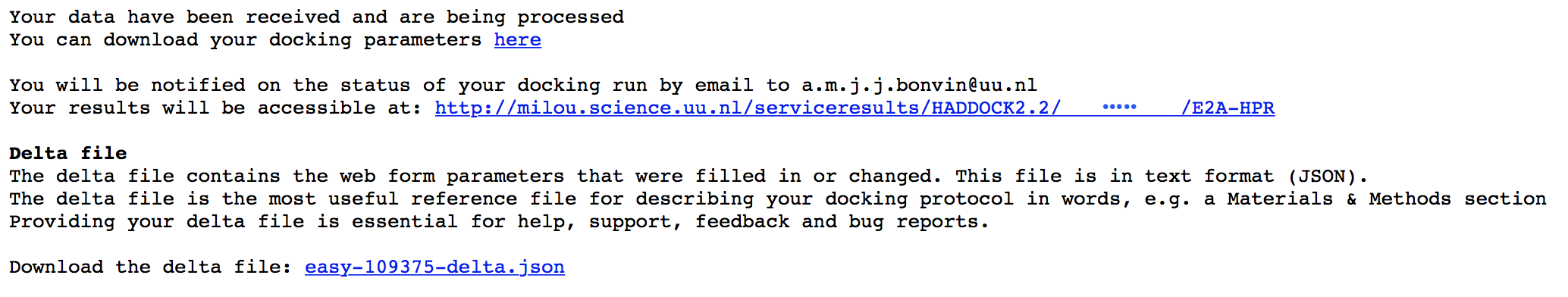
We strongly recommend to save this haddockparameter file since it will allow you to repeat the run by simple upload into the file upload inteface of the HADDOCK webserver. It can serve as input reference for the run. This file can also be edited to change a few parameters for examples. An excerpt of this file is shown here:
HaddockRunParameters (
  runname = 'Cathepsin-ligand',
  auto_passive_radius = 6.5,
  create_narestraints = True,
  delenph = False,
  ranair = False,
  cmrest = False,
  kcont = 1.0,
  surfrest = False,
  ksurf = 1.0,
  noecv = True,
  ncvpart = 2.0,
  structures_0 = 1000,
  ntrials = 5,
...
Click now on the link to the results page. While your input data are being validated and processed the page will show:
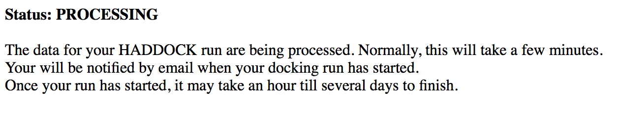
During this stage the PDB and eventually provided restraint files are being validated. Further the server makes use of Molprobity to check side-chain conformations, eventually swap them (e.g. for asparagines) and define the protonation state of histidine residues. Once this has been successfully done, the page will indicated that your job is first QUEUED, and then RUNNING.
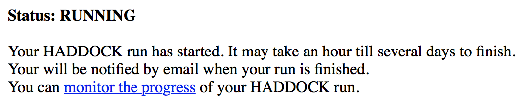
The page will automatically refresh and the results will appear upon completions (which can take between 1/2 hour to several hours depending on the size of your system and the load of the server). You will be notified by email once your job has successfully completed.
Analysis of the results
Once your run has completed you will be presented with a result page showing the cluster statistics and some graphical representation of the data (and if registered, you will also be notified by email). If using course credentials provided to you, the number of models generated will have been decreased to allow the runs to complete within a reasonable amount of time.
We already pre-calculated full docking run for both ensembles (we slightly increased the default number of models generated at each stage of HADDOCK: 4000 for rigid-body docking and 400 for semi-flexible and water refinement). Only the best (in term of HADDOCK score) 200 models generated at the water refinement stage of HADDOCK were further selected for analysis. The full runs for both “bemeta” and “apoMD” ensemble can be accessed at:
- bemeta_ensemble: View here the pre-calculated results
- apoMD_ensemble: View here the pre-calculated results
Inspect the result pages. How many clusters are generated?
Note: The bottom of the page gives you some graphical representations of the results, showing the distribution of the solutions for various measures (HADDOCK score, van der Waals energy, …) as a function of the RMSD from the best generated model (the best scoring model).
The ranking of the clusters is based on the average score of the top 4 members of each cluster. The score is calculated as:
HADDOCKscore = 1.0 Evdw + 0.1 Eelec + 1.0 Edesol + 0.1 Eair
where Evdw is the intermolecular van der Waals energy, Eelec the intermolecular electrostatic energy, Edesol represents an empirical desolvation energy term adapted from Fernandez-Recio et al. J. Mol. Biol. 2004, and Eair the AIR energy. The cluster numbering reflects the size of the cluster, with cluster 1 being the most populated cluster. The various components of the HADDOCK score are also reported for each cluster on the results web page.
Consider the cluster scores and their standard deviations. Is the top ranked cluster significantly better than the second one? (This is also reflected in the z-score).
In case the scores of various clusters are within standard devatiation from each other, all should be considered as a valid solution for the docking. Ideally, some additional independent experimental information should be available to decide on the best solution.
Visualisation of docked models
Let’s now visualise the various solutions!
Then start PyMOL and load the best clusters representatives:
File menu -> Open -> Select the files …
Repeat this for each cluster. Once all files have been loaded, type in the PyMOL command window:
load ~/Tutorials/metaHADDOCK/tutorial_files/apoMD/holo_GLUCO.pdb
as cartoon
util.cnc
The reference We now want to highlight the ligand in sticks. In the reference structure, the ligand belong to chain A and has the residue number 400. To allow RMSD calculations, we first need to change the residue number, chainID and segid of the ligand in the reference structure:
At last, we can remove water molecules (reference structure) and hydrogens to facilitate the visual comparison with the reference structure.
show sticks, resn UDP
remove hydrogens
remove resn HOH
Let’s then superimpose all models on the reference structure holo_GLUCO and calculate the ligand RMSD:
align bemeta_cluster1_1, holo_GLUCO
rms_cur resn UDP and holo_GLUCO, resn UDP and bemeta_cluster1_1
Repeat this for the various cluster representatives and take note of the ligand RMSD values
See solution:
 * bemeta cluster2_1     HADDOCKscore [a.u.] = -47.2 +/- 1.4       ligand-RMSD = 7.48Å
 * bemeta cluster1_1     HADDOCKscore [a.u.] = -44.1 +/- 2.2       ligand-RMSD = 0.79Å
 * apoMD cluster3_1      HADDOCKscore [a.u.] = -32.4 +/- 2.0       ligand-RMSD = 7.86Å
 * apoMD cluster2_1      HADDOCKscore [a.u.] = -26.2 +/- 1.2       ligand-RMSD = 7.48Å
 * apoMD cluster1_1      HADDOCKscore [a.u.] = -24.9 +/- 0.9       ligand-RMSD = 3.98Å
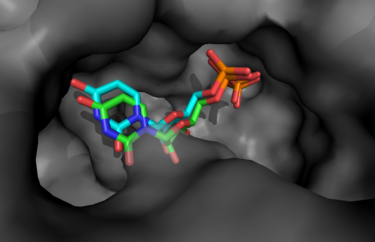
If you want to take a look at the best solution generated by HADDOCK, unfold the menu below:
See a view of the top model of cluster1 for bemeta (in cyan), superimposed on the reference structure (1jg6 in green):
Congratulations!
You have completed this tutorial. If you have any questions or suggestions, feel free to post on the dedicated topic on our interest group forum.
References
[1]: Laio and Parrinello, PNAS October 1, 2002. 99 (20) 12562-12566
[2]: Huang and Zou, Proteins. 2007 Feb 1;66(2):399-421
[3]: Forli, Molecules 2015, 20, 18732-18758
[4]: Mandal et al., Eur J Pharmacol. 2009 Dec 25;625(1-3):90-100
[5]: Sliwoski et al., Pharmacol Rev. 2013 Dec 31;66(1):334-95
[6]: Chen, Trends Pharmacol Sci. 2015 Feb;36(2):78-95
[7]: Koshland D. E. PNAS 1958, 44, 98-104
[8]: Teague, Nat Rev Drug Discov. 2003 Jul;2(7):527-41
[9]: G.C.P van Zundert et al., J. Mol. Biol., 2015, 428, 720-725
[10]: Pronk et al. Bioinf, 29 (2013), pp. 845-854
[11]: Deserno and Holm, J. Chem. Phys. 109, (1998) 7678
[12]: Laio et al., J. Phys. Chem. B, 2005, 109 (14), pp 6714–6721
[13]: Bussi et al., Phys. Rev. Lett. 2006, 96, 090601
[14]: Laio and Gervasio, Reports on Progress in Physics (2008), Vol 71, Num 12
[15]: Barducci et al., Phys. Rev. Lett. 2008, 100, 020603
[16]: Piana and Laio., J. Phys. Chem. B, 2007, 111 (17), pp 4553–4559
[17]: Tribello et al., Comput. Phys. Commun. 185, 604 (2014)
[18]: Gervasio et al., J Am Chem Soc. 2005 Mar 2;127(8):2600-7
[19]: Vargiu et al., Nucleic Acids Res. 2008 Oct; 36(18): 5910–5921
[20]: Shao et al., J. Chem. Theory Comput. 2007, 3, 2312-2334