User manual
There are a few default parameters listed below that come with the
standard powerfit command. These default parameters are also the
standard in the PowerFit webserver.
Below we will describe the different parameters and some input examples.
In addition we also explain the output of the report.html
file or result page on the webserver.
powerfit <map> <resolution> <pdb>
# To generate the report page after the run:
powerfit <map> <resolution> <pdb> --report --delimiter ','
Parameters
Rotational sampling interval (-a): Rotational sampling density in degrees. Increasing this number by a factor of 2 results in approximately 8 times more rotations sampled.
Chain ID(s) (-c): The chain IDs of the structure to be fitted. Multiple chains can be selected using a comma separated list, i.e. A,B,C. The default is the whole structure.
Laplace pre-filter (-nl): Usage of the Laplace pre-filter to filter the density data.
Can be combined with the core-weighted local cross-correlation. In the default this
is turned on and can be disabled by selecting Disable Laplace pre-filter in the
webserver or using the -nl flag on the command line.
Core-weighted local cross-correlation (-ncw): Usage of a core-weighted local cross-correlation
score. It can be combined with the Laplace pre-filter. In the default
this is turned on and can be disabled by selecting Disable Core-weighted correlation
in the webserver or using the -ncw flag on the command line.
Number of top solutions (-n): Number of top solutions for which the model in the coordinate frame of the density map will be returned. This number will be capped if less solutions are found as requested. The default is 10.
Density map resampling (-nr): Resample the density map prior to fitting. In the default
this is turned on and can be disabled by selecting No resampling in the webserver or using
the -nr flag on the command line.
Resampling rate (-rr): Adjust resampling of the density map to a specific factor of the Nyquist rate. The default is 2.
Density map trimming (-nt): Trim the density to a preddefined intensity cutoff.
In the default this is turned on and can be disabled by selecting No trimming in
the webserver or using the -nt flag on the command line.
Trimming cutoff (-tc): Intensity cutoff to which the map will be trimmed. Default is 10 percent of the maximum intensity.
In most cases the default parameters of PowerFit will be reasonable and don't have to be changed. In cases where the fitting results are unsatisfactory, improvements might be achieved by disabling the Laplace pre-filter, disabling the core-weighted correlation, or increasing the rotational samping. Increasing rotational sampling by a factor of 2 results in approximately 8 times more rotations and thus a signigicant increase in the runtime of a job.
Input examples
First, to see all options and their descriptions type
powerfit --help
To perform a search with an approximate 24° rotational sampling interval with laplace pre-filtering and core-weighted scoring function using 1 CPU
powerfit <map> <resolution> <pdb> -a 24
To use multiple CPU cores without laplace pre-filter and 5° rotational interval
powerfit <map> <resolution> <pdb> -p 4 -nl -a 5
To off-load computations to the GPU and do not use the core-weighted scoring function and write out the top 15 solutions
powerfit <map> <resolution> <pdb> -g -ncw -n 15
Note that all options can be combined except for the -g and -p flag:
calculations are either performed on the CPU or GPU.
To run on GPU
powerfit <map> <resolution> <pdb> --gpu
...
Using GPU-accelerated search.
...
--help if you have multiple GPUs and want to specify which one to use)
Output
When the search is finished, several output files are created. These output files can be downloaded from the result page when run on the webserver and are automatically created and saved when run using the CLI.
- fit_N.pdb: the top N best fits.
- solutions.out: all the non-redundant solutions found, ordered by their correlation score. The first column shows the rank, column 2 the correlation score, column 3 and 4 the Fisher z-score and the number of standard deviations (see N. Volkmann 2009, and Van Zundert and Bonvin 2016); column 5 to 7 are the x, y and z coordinate of the center of the chain; column 8 to 17 are the rotation matrix values.
- lcc.mrc: a cross-correlation map, showing at each grid position the highest correlation score found during the rotational search.
- powerfit.log: a log file, including the input parameters with date and timing information.
- report.html and state.mvsj: an HTML report and its MolViewSpec with interactive 3D visualization of the best fits.
Only written if the
--report --delimiter ,arguments are passed.
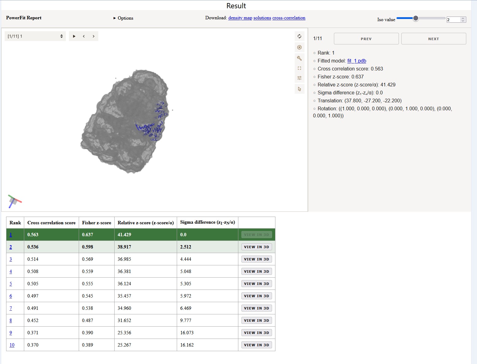
Report page
At the top of the report page is an interactive MolViewSpec with 3D visualization of the best fits. It shows the best 15 non-redundant solutions found by PowerFit as reported in the solutions.out file. While clicking through the different models, the viewer reports the rank, cross correlation score, Fisher z-score, and Sigma difference. When opening the Options dropdown you can see which parameters where used for the fitting.
Solutions table
The table below the interactive viewer reports the values of the models in one overview. In a previous investigation we fitted 379 individual chains in 6 ribosome cryo-EM density maps starting at a resolution of 6Å up to 30Å. Successful fits were obtained in >99% of the cases for which the difference in error-normalized z-score between the two top scoring solutions was larger than ~2.5. Conversely, in less than 3% of the failed cases did the difference exceed one. Van Zundert and Bonvin 2016
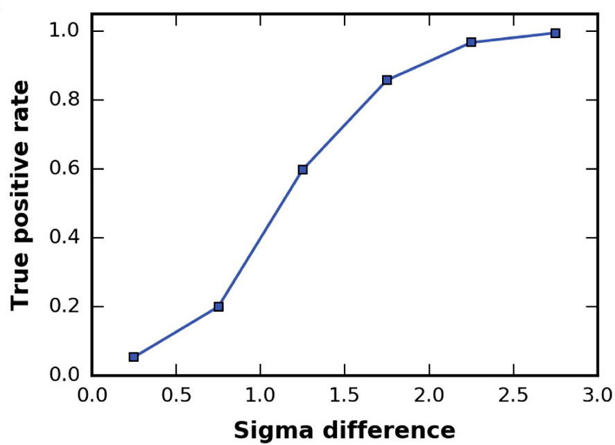 The true-positive rate is given versus the difference in Fisher z-score standard deviations
between the top 2 solutions. The fitting results were binned in 6 bins, starting from 0 to 3
sigma with a step size of 0.5.
The true-positive rate is given versus the difference in Fisher z-score standard deviations
between the top 2 solutions. The fitting results were binned in 6 bins, starting from 0 to 3
sigma with a step size of 0.5.
To enhance the interpretation of the results, the entries in the table are colored in a green gradient up to a sigma difference of 3. Coloring is however only applied if the sigma difference to Fit 10 is below 3 in order to avoid higlighting runs with no distinction between the fits. Note that in case of symmetrical complexes multiple equally well scoring fits might be reported.