

Tutorial describing the use of a local version of HADDOCK2.4
This tutorial consists of the following sections:
- Introduction
- Setup/Requirements
- HADDOCK general concepts
- Installing HADDOCK
- Preparing PDB files for docking
- Defining restraints for docking
- Setting up the docking
- Analysing the docking results
- Congratulations!
Introduction
This tutorial will demonstrate the use of a local installation of HADDOCK2.4 for predicting the structure of biomolecular complexes. It will cover various steps, from the installation of a local HADDOCK2.4 version and the third party software required, the preparation of PDB files for docking, the definition of restraints to guide the docking, the setup of the docking and finally the analysis of the results. General information about HADDOCK can be found on our group page and its corresponding online manual. Also take note of the HADDOCK online forum where you can post HADDOCK-related questions and search the archive for possible answers.
Throughout the tutorial, colored text will be used to refer to questions or instructions, and/or PyMOL commands.
This is a question prompt: try answering it! This an instruction prompt: follow it! This is a PyMOL prompt: write this in the PyMOL command line prompt! This is a Linux prompt: insert the commands in the terminal!
Setup/Requirements
In order to follow this tutorial you will need to work on a Linux or MaxOSX system. We will also make use of PyMOL (freely available for most operating systems) on your computer in order to visualize the input and output data. We will provide you links to download the various required software and data.
HADDOCK general concepts
HADDOCK (see https://www.bonvinlab.org/software/haddock2.4) is a collection of python scripts derived from ARIA (https://aria.pasteur.fr) that harness the power of CNS (Crystallography and NMR System – https://cns-online.org) for structure calculation of molecular complexes. What distinguishes HADDOCK from other docking software is its ability, inherited from CNS, to incorporate experimental data as restraints and use these to guide the docking process alongside traditional energetics and shape complementarity. Moreover, the intimate coupling with CNS endows HADDOCK with the ability to actually produce models of sufficient quality to be archived in the Protein Data Bank.
A central aspect to HADDOCK is the definition of Ambiguous Interaction Restraints or AIRs. These allow the translation of raw data such as NMR chemical shift perturbation or mutagenesis experiments into distance restraints that are incorporated in the energy function used in the calculations. AIRs are defined through a list of residues that fall under two categories: active and passive. Generally, active residues are those of central importance for the interaction, such as residues whose knockouts abolish the interaction or those where the chemical shift perturbation is higher. Throughout the simulation, these active residues are restrained to be part of the interface, if possible, otherwise incurring in a scoring penalty. Passive residues are those that contribute for the interaction, but are deemed of less importance. If such a residue does not belong in the interface there is no scoring penalty. Hence, a careful selection of which residues are active and which are passive is critical for the success of the docking.
The docking protocol of HADDOCK was designed so that the molecules experience varying degrees of flexibility and different chemical environments, and it can be divided in three different stages, each with a defined goal and characteristics:
-
1. Randomization of orientations and rigid-body minimization (it0)
In this initial stage, the interacting partners are treated as rigid bodies, meaning that all geometrical parameters such as bonds lengths, bond angles, and dihedral angles are frozen. The partners are separated in space and rotated randomly about their centers of mass. This is followed by a rigid body energy minimization step, where the partners are allowed to rotate and translate to optimize the interaction. The role of AIRs in this stage is of particular importance. Since they are included in the energy function being minimized, the resulting complexes will be biased towards them. For example, defining a very strict set of AIRs leads to a very narrow sampling of the conformational space, meaning that the generated poses will be very similar. Conversely, very sparse restraints (e.g. the entire surface of a partner) will result in very different solutions, displaying greater variability in the region of binding.See animation of rigid-body minimization (it0):
-
2. Semi-flexible simulated annealing in torsion angle space (it1)
The second stage of the docking protocol introduces flexibility to the interacting partners through a three-step molecular dynamics-based refinement in order to optimize interface packing. It is worth noting that flexibility in torsion angle space means that bond lengths and angles are still frozen. The interacting partners are first kept rigid and only their orientations are optimized. Flexibility is then introduced in the interface, which is automatically defined based on an analysis of intermolecular contacts within a 5Å cut-off. This allows different binding poses coming from it0 to have different flexible regions defined. Residues belonging to this interface region are then allowed to move their side-chains in a second refinement step. Finally, both backbone and side-chains of the flexible interface are granted freedom. The AIRs again play an important role at this stage since they might drive conformational changes.See animation of semi-flexible simulated annealing (it1):
-
3. Refinement in Cartesian space with explicit solvent (water)
The final stage of the docking protocol immerses the complex in a solvent shell so as to improve the energetics of the interaction. HADDOCK currently supports water (TIP3P model) and DMSO environments. The latter can be used as a membrane mimic. In this short explicit solvent refinement the models are subjected to a short molecular dynamics simulation at 300K, with position restraints on the non-interface heavy atoms. These restraints are later relaxed to allow all side chains to be optimized.See animation of refinement in explicit solvent (water):
The performance of this protocol of course depends on the number of models generated at each step. Few models are less probable to capture the correct binding pose, while an exaggerated number will become computationally unreasonable. The standard HADDOCK protocol generates 1000 models in the rigid body minimization stage, and then refines the best 200 – regarding the energy function - in both it1 and water. Note, however, that while 1000 models are generated by default in it0, they are the result of five minimization trials and for each of these the 180º symmetrical solution is also sampled. Effectively, the 1000 models written to disk are thus the results of the sampling of 10.000 docking solutions.
The final models are automatically clustered based on a specific similarity measure - either the positional interface ligand RMSD (iL-RMSD) that captures conformational changes about the interface by fitting on the interface of the receptor (the first molecule) and calculating the RMSDs on the interface of the smaller partner, or the fraction of common contacts (current default) that measures the similarity of the intermolecular contacts. For RMSD clustering, the interface used in the calculation is automatically defined based on an analysis of all contacts made in all models.
Installing HADDOCK
Downloading HADDOCK
In this tutorial we will make use of the new HADDOCK2.4 version.
To obtain HADDOCK2.4 fill the HADDOCK license form.
Downloading CNS
The other required piece of software to run HADDOCK is its computational engine, CNS (Crystallography and NMR System – https://cns-online.org ). CNS is freely available for non-profit organisations. In order to get access to all features of HADDOCK you will need to recompile CNS using the additional files provided in the HADDOCK distribution in the cns1.3 directory. Compilation of CNS might be non-trivial. We are providing some instructions here. Consult also for some guidance the related entry in the HADDOCK forum
Untar the archive in the software directory.
Auxiliary software
FreeSASA. In order to identify surface-accessible residues to define restraints for HADDOCK we can make use of NACCESS freely available to non-profit users, or its open-source software alternative FreeSASA. We will here make use of FreeSASA. Following the download and installation instructions from the FreeSASA website. The direct download command is:
cd
mkdir software
cd software
wget https://freesasa.github.io/freesasa-2.1.2.tar.gz
If running into problems you might want to disable json and xml support. Here we will assume you save the tar archive under the software directory in your home directory:
HADDOCK-tools: A collection of HADDOCK-related scripts freely available from our GitHub repository. To install it:
cd ~/software
git clone https://github.com/haddocking/haddock-tools
In case git is not installed on your system, go the GitHub site given in the command and download directly the archive.
MolProbity: MolProbity is a structure validate software suite developed in the Richardson lab at Duke University. In the context of HADDOCK we are making use of MolProbity to define the protonation state of Histidine residues using the reduce application. An pre-compiled executable can be freely downloaded from the MolProbity GitHub website. You can directly download the reduce executable for Linux or OSX.
Put the executable in ~software/bin, rename it to reduce if needed and make sure it is executable (e.g. chmod +x ~/software/bin/reduce).
PDB-tools: A useful collection of Python scripts for the manipulation (renumbering, changing chain and segIDs…) of PDB files is freely available from our GitHub repository. To install it:
cd ~/software
git clone https://github.com/haddocking/pdb-tools
In case git is not installed on your system, go the GitHub site given in the command and download directly the archive.
ProFit: ProFit is designed to be the ultimate protein least squares fitting program. Some of the provided analysis tools in HADDOCK make use of Profit. Profit can be obtained free of charge for both non-profit and commercial users. The latter should notify the authors that they are using it. For information and download see the ProFit webpage.
PyMol: We will make use of PyMol for visualisation. If not already installed on your system, download and install PyMol.
At this point we will assume that you successfully downloaded all auxiliary software and installed the executables (or links to them) in ~/software/bin
If running under bash shell, type:
And for csh:
Configuring HADDOCK
After having downloaded HADDOCK from the above link, unpack the archive under the ~/software directory with the following command:
HADDOCK2.4 version requires python version 2.7 and CNS version 1.3 (see above for CNS installation instructions). Importantly, python2 (pointing to python2.7) should be existing on your system. / As python2.7 is end of life, one way to install it is to use miniconda on your system.
Once miniconda has been installed and activated, create a HADDOCK2.4 environment with the following command (withing the haddock2.4 directory):
conda env create -f requirements.yml
Then activate the haddock2.4 environment with:
This configuration file should contain the following information:
CNSTMP defining the location of your CNS executable
QUEUETMP defining the submission command for running the jobs (e.g. either via csh or through a specific command submitting to your local batch system)
NUMJOB defining the number of concurrent jobs executed (or submitted).
QUEUESUB defining the HADDOCK python script used to run the jobs (the default QueueSubmit_concat.py should do in most cases).
And example configuration file for running on local resources assuming a 4 core system would be:
  set CNSTMP=/home/software/cns/cns_solve-1.31-UU-Linux64bits.exe
  set QUEUETMP=/bin/csh
  set NUMJOB=4
  set QUEUESUB=QueueSubmit_concat.py
For submitting to a batch system instead you might want to use a wrapper script. An example for torque can be found here.
In order to configure HADDOCK, call the install.csh script with as argument the configuration script you just created:
./install.csh <my-config-file>
There is one more file that should be manually edited to define the number of models to concatenate within one job (useful when submitting to a batch system to ensure jobs are not too short in queue). Depending on the size of your system, a typical run time for rigid body docking would be a few tens of seconds per model written to disk (which effectively correspond to 10 docking trials internally), and a few minutes per model for the flexible refinement and the final refinement. But this can increase a lot depending on the complexity of your system and the number of molecules to dock.
jobconcat["0"] = 5
jobconcat["1"] = 1
jobconcat["2"] = 1
If running on local system, change all values to 1.
One last command to source the HADDOCK environment (under bash) (for csh, replace .sh by .csh):
cd ~/software/haddock2.4
source ./haddock_configure.sh
At this stage you should be ready to use HADDOCK2.4!
Preparing PDB files for docking
In this section we describe some basic points in preparing PDB files for HADDOCK. First of all, each PDB file must end with an END statement.
We will illustrate here three aspects:
- Cleaning PDB files prior to docking
- Introducing a mutation in a PDB file
- Dealing with an ensemble of models
- Dealing with multi-chain proteins
We suggest to create separate directories for the different cases and work from those.
Cleaning PDB files prior to docking
We will use here as example the E2A structure used as input in our HADDOCK webserver basic protein-protein docking tutorial. This protein is part of a phospho-transfer complex and one of its histidine residue should in principle be phosphorylated. Start PyMOL and in the command line window of PyMOL (indicated by PyMOL>) type:
show cartoon
hide lines
show sticks, resn HIS
You should see a backbone representation of the protein with only the histidine side-chains visible. Try to locate the histidines in this structure.
Is there any phosphate group present in this structure?
Note that you can zoom on the histidines by typing in PyMOL:
Revert to a full view with:
As a preparation step before docking, it is advised to remove any irrelevant water and other small molecules (e.g. small molecules from the crystallisation buffer), however do leave relevant co-factors if present. For E2A, the PDB file only contains water molecules. You can remove those in PyMOL by typing:
As final step save the molecule as a new PDB file which we will call: e2a_1F3G.pdb
For this in the PyMOL command line type:
Note that you can of course also simply edit the PDB file with your favorite text editor.
Since the biological function of the E2A-HPR complex is to transfer a phosphate group from one protein to another, via histidines side-chains, it is relevant to make sure that a phosphate group be present for docking. As we have seen above none is currently present in the PDB files. HADDOCK does support a list of modified amino acids which you can find at the following link: https://wenmr.science.uu.nl/haddock2.4/library.
Check the list of supported modified amino acids. What is the proper residue name for a phospho-histidine in HADDOCK?
In order to use a modified amino-acid in HADDOCK, the only thing you will need to do is to edit the PDB file and change the residue name of the amino-acid you want to modify. Don’t bother deleting irrelevant atoms or adding missing ones, HADDOCK will take care of that. For E2A, the histidine that is phosphorylated has residue number 90. In order to change it to a phosphorylated histidine do the following:
Edit the PDB file (e2a_1F3G.pdb) in your favorite editor Change the name of histidine 90 to NEP Save the file (as simple text file) under a new name, e.g. e2aP_1F3G.pdb
Note: The same procedure can be used to introduce a mutation in an input protein structure.
Note: In the haddock-tools scripts that you installed, there is a python script called pdb_mutate.py that allows you to introduce such a mutation from the command line (call the script without arguments to see its usage):
pdb_mutate.py e2a_1F3G.pdb A 90 HIS NEP >e2aP_1F3G.pdb
Prior to using this file in HADDOCK is to remove any chainID and segID information. This can easily be done using our pdb-tools scripts:
pdb_chain.py e2aP_1F3G.pdb | ~/software/pdb-tools/pdb_seg.py >e2aP_1F3G-clean.pdb
In case your PDB file comes from some modelling software, it might be good to check that it is properly formatted. This can be done with our pdb-tools script:
pdb_validate.py e2aP_1F3G-clean.pdb
Note that not all warnings are relevant. The important part is that the columns be properly aligned.
You can also check if your PDB model has gaps in the structure. If gaps are detected you can either try to modell the missing fragments, or define a few distance restraints to keep the fragments together during docking (see the section about Dealing with multi-chain proteins.
pdb_gap.py e2aP_1F3G-clean.pdb
Another possible issue with the starting PDB structures can be double occupancy of some side-chains. This is quite common in high resolution crystal structures.
For HADDOCK, you will have to remove those double occupancies (or create multiple models corresponding to various conformations). A simply way to get rid of double occupancies (only the first occurence of each side-chain will be kept) is to use our pdb-tools pdb_selaltloc.py script.
Dealing with an ensemble of models
HADDOCK can take as input an ensemble of conformation. This has the advantage that it allows to pre-sample possible conformational changes. We however recommend to limit the number of conformers used for docking, since the number of conformer combinations of the input molecules might explode (e.g. 10 conformers each will give 100 starting combinations, and if we generate 1000 rigid body models (see HADDOCK general concepts above) each combination will only be sampled 10 times).
While the HADDOCK webportal will take those as an ensemble PDB file (with MODEL / ENDMDL statements), the local version of HADDOCK expects those models to be provided as single structure and an additional file providing a listing of the models. To illustrate this we will use the HPR protein used as input in our HADDOCK2.4 webserver basic protein-protein docking tutorial. The input structure for docking corresponds to an NMR ensemble of 30 models.
We will now inspect the HPR structure. For this start PyMOL and in the command line window of PyMOL type:
show cartoon
set all_states, on
You should now be seeing the 30 conformers present in this NMR structure.
Save the molecule as a new PDB file which we will call: hpr_1HDN.pdb
For this in the PyMOL command line window type:
As in the previous example, make sure to remove all chainID and segidID from the PDB file
pdb_chain.py hpr_1HDN.pdb | pdb_seg.py >hpr_1HDN-clean.pdb
While this file would be ready for upload to the HADDOCK server, we need to split the models into individual files for use with the local version of HADDOCK.
Again, this can be done easily with one of our pdb-tools script:
pdb_splitmodel.py hpr_1HDN-clean.pdb
The result of this are 30 separate PBD models named hpr_1HDN-clean_XX.pdb where XX is the model number. To use this ensemble of models we need to create a text file listing those models. This can be done for example with the following command (using in this example only the top10 models):
\ls -1 hpr_1HDN-clean_*.pdb | awk '{print $1}' >hpr_1HDN.list
\ls -rt hpr_1HDN-clean_*.pdb | head -10 > hpr_1HDN_1.list
Dealing with multi-chain proteins
It can happen that one of your molecule consists of multiple chains, such as for example a homo-dimer or an antibody structure. HADDOCK can in principle handle those, but it is important that there is not overlap in the residue numbering between the chains since the molecule will be assigned a single chainID/segID for docking. As an example we will consider an antibody structure (PDB entry 4G6K).
show cartoon
hide lines
remove resn HOH
This structure consists of two chains, L and H, with overlapping residue numbering. Turn on the sequence in PyMol (under the Display menu) and find out what is the last residue number of the first chain L. We need this information to know by how much we should shift the numbering of the second chain H.
Save the molecule as a PDB file:
We will now shift the numbering of chain L to avoid overlap in numbering. This can easily be done using our pdb-tools scripts. The first chain ends with residue number 212 and the second chain starts at 1. We will shift the numbering of the second chain by 500 to avoid numbering overlap:
We added a TER statement between the chains and an END statement at the end of the file.
Note that this structure consists of two separate chains. It will therefore be important to define a few distance restraints to keep them together during the high temperature flexible refinement stage of HADDOCK. This can easily be done using another script from haddock-tools:
restrain_bodies.py 4G6K-clean.pdb >antibody-unambig.tbl
The result file contains two CA-CA distance restraints with the exact distance measured between the picked CA atoms:
  assign (segid  and resi 189 and name CA) (segid  and resi 693 and name CA) 21.023 0.0 0.0
  assign (segid  and resi 116 and name CA) (segid  and resi 702 and name CA) 44.487 0.0 0.0
Note that in this example, we are missing segment identifiers since they were not present in the PDBs. And if they are present, make sure those match what you are going to define as segIDs in HADDOCK. So in this case we need to add A for the first molecule and B for the second:
  assign (segid A and resi 189 and name CA) (segid B and resi 693 and name CA) 21.023 0.0 0.0
  assign (segid A and resi 116 and name CA) (segid B and resi 702 and name CA) 44.487 0.0 0.0
This is the file you should save as unambig.tbl and pass to HADDOCK.
Defining restraints for docking
Before setting up the docking we need first to generate distance restraint files in a format suitable for HADDOCK. HADDOCK uses CNS as computational engine. A description of the format for the various restraint types supported by HADDOCK can be found in our Nature Protocol paper, Box 4.
Distance restraints are defined as:
assi (selection1) (selection2) distance, lower-bound correction, upper-bound correction
The lower limit for the distance is calculated as: distance minus lower-bound correction
and the upper limit as: distance plus upper-bound correction.
The syntax for the selections can combine information about chainID - segid keyword -, residue number - resid
keyword -, atom name - name keyword.
Other keywords can be used in various combinations of OR and AND statements. Please refer for that to the online CNS manual.
We will shortly explain in this section how to generate both ambiguous interaction restraints (AIRs) and specific distance restraints for use in HADDOCK illustrating three scenarios:
- Interface mapping on both side (e.g. from NMR chemical shift perturbation data)
- Specific distance restraints (e.g. cross-links detected by MS)
- Interface mapping on one side, full surface on the other
Information about various types of distance restraints in HADDOCK can also be found in our online manual pages.
Defining AIRs from interface mapping
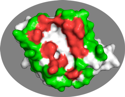
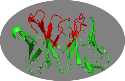
We will use as example here the NMR chemical shift perturbations from the E2A-HPR complex used in our HADDOCK 2.4 webserver basic protein-protein docking tutorial. The following residues of E2A were identified by Wang et al, EMBO J (2000) as having significant chemical shift perturbations:
38,40,45,46,69,71,78,80,94,96,141
Let’s visualize them in PyMOL using the clean PDB file we created in the Cleaning PDB files prior to docking section of this tutorial:
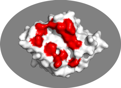
Inspect the surface.
Do the identified residues form a well defined patch on the surface? Do they form a contiguous surface?
The answer to the last question should be no: We can observe residue in the center of the patch that do not seem significantly affected while still being in the middle of the defined interface. This is the reason why in HADDOCK we also define “passive” residues that correspond to surface neighbors of active residues. These should be selected manually, filtering for solvent accessible residues (the HADDOCK server will do it for you).
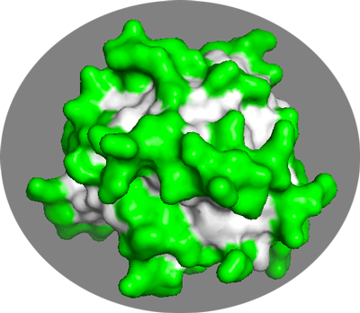
A list of passive residues the server would select in this case is:
35,37,39,42,43,44,47,48,64,66,68,72,73,74,82,83,84,86,97,99,100,105,109,110,112,131,132,133,143,144
In the same PyMol session as before you can visualize them with:
In general it is better to be too generous rather than too strict in the definition of passive residues.
And important aspect is to filter both the active (the residues identified from your mapping experiment) and passive residues by their solvent accessibility. Our webserver uses a default relative accessibility of 15% as cutoff. This is not a hard limit. You might consider including even more buried residues if some important chemical group seems solvent accessible from a visual inspection.
We can use freesasa to calculate the residue solvent accessibilities:
freesasa e2a_1F3G.pdb --format=rsa >e2a_1F3G.rsa
The results is file similar to the output of naccess containing the per residue solvent accessibilities, both absolute and relative values, also distinguishing between backbone and side-chains:
REM  FreeSASA 2.1.2
REM  Absolute and relative SASAs for e2a_1F3G.pdb
REM  Atomic radii and reference values for relative SASA: ProtOr
REM  Chains: A
REM  Algorithm: Lee & Richards
REM  Probe-radius: 1.40
REM  Slices: 20
REM RES _ NUM      All-atoms   Total-Side   Main-Chain    Non-polar    All polar
REM                ABS   REL    ABS   REL    ABS   REL    ABS   REL    ABS   REL
RES THR A  19   125.49  89.3  59.11  59.9  66.38 158.2  33.47  45.0  92.02 139.1
RES ILE A  20    29.18  16.6  23.16  17.3   6.02  14.5  29.18  21.0   0.00   0.0
RES GLU A  21    63.92  36.7  50.29  38.0  13.63  32.5  13.71  26.5  50.21  41.0
RES ILE A  22     0.00   0.0   0.00   0.0   0.00   0.0   0.00   0.0   0.00   0.0
RES ILE A  23    25.26  14.4  25.26  18.8   0.00   0.0  25.26  18.2   0.00   0.0
...
The following command will return all residues with a relative SASA for either the backbone or the side-chain > 15%:
awk '{if (NF==13 && $5>40) print $0; if (NF==14 && $6>40) print $0}' e2a_1F3G.rsa
Once you have defined your active and passive residues for both molecules, you can proceed with the generation of the AIR restraint file for HADDOCK.
For this you can either make use of our online Generate Restraints haddock-restraints web service, entering the list of active and passive residues for each molecule, and saving the resulting restraint list to a text file, or use another haddock-tools script.
To use our haddock-tools active-passive-to-ambig.py script you need to create for each molecule a file containing two lines:
- The first line corresponds to the list of active residues (numbers separated by spaces)
- The second line corresponds to the list of passive residues.
For our E2A-HPR example this would be:
- For E2A (a file called e2a-act-pass.list):
38 40 45 46 69 71 78 80 94 96 141
35 37 39 42 43 44 47 48 64 66 68 72 73 74 82 83 84 86 97 99 100 105 109 110 112 131 132 133 143 144
- and for HPR (a file called hpr-act-pass.list):
15 16 17 20 48 49 51 52 54 56
9 10 11 12 21 24 25 34 37 38 40 41 43 45 46 47 53 55 57 58 59 60 84 85
Using those two file we can generate the CNS-formatted AIR restraint files with the following command:
active-passive-to-ambig.py e2a-act-pass.list hpr-act-pass.list >e2a-hpr-ambig.tbl
This generates a file called e2a-hpr-ambig.tbl that contains the AIR restraints. The default distance range for those is between 0 and 2Å, which might seem short but makes senses because of the 1/r^6 summation in the AIR energy function that makes the effective distance be significantly shorter than the shortest distance entering the sum.
The effective distance is calculated as the SUM over all pairwise atom-atom distance combinations between an active residue and all the active+passive on the other molecule: SUM[1/r^6]^(-1/6).
If you modify this file, it is possible to quickly check if the format is valid. To do so, you can find in the haddock-tools repository a folder named haddock_tbl_validation that contains a script called validate_tbl.py. To use it, simply run:
python ~/software/haddock-tools/haddock_tbl_validation/validate_tbl.py --silent e2a-hpr-ambig.tbl
No output means that your TBL file is valid. You can also find TBL file examples for different types of restraints in the haddock-tools/haddock_tbl_validation/ directory.
Defining specific distance restraints
You can define in HADDOCK unambiguous distance restraints between specific pairs of atoms to define restraints coming for example from MS cross-linking experiments or DEER experiments. As an illustration we will use cross-links from our HADDOCK cross-links tutorial obtained for the complex between PRE5 (UniProtKB: O14250) and PUP2 (UniProtKB: Q9UT97). From MS, we have seven experimentally determined cross-links (4 ADH & 3 ZL) (Leitner et al., 2014), which we will define as CA-CA distance restraints (restraints.txt):
# ADH crosslinks
A  27 CA B  18 CA 0 23
A 122 CA B 125 CA 0 23
A 122 CA B 128 CA 0 23
A 122 CA B 127 CA 0 23

# ZL crosslinks
A 55 CA B 169 CA 0 26
A 55 CA B 179 CA 0 26
A 54 CA B 179 CA 0 26
This is the format used by our DisVis portal to represent the cross-links. Each cross-link definition consists of eight fields:
- chainID of the 1st molecule
- residue number
- atom name
- chainID of the 2nd molecule
- residue number
- atom name
- lower distance limit
- upper distance limit
The corresponding CNS-formatted HADDOCK restraint file for those would be (unambig-xlinks.tbl):
assign (segid A and resid 27  and name CA) (segid B and resid 18  and name CA)  23 23 0
assign (segid A and resid 122 and name CA) (segid B and resid 125 and name CA)  23 23 0
assign (segid A and resid 122 and name CA) (segid B and resid 128 and name CA)  23 23 0
assign (segid A and resid 122 and name CA) (segid B and resid 127 and name CA)  23 23 0
assign (segid A and resid 55  and name CA) (segid B and resid 169 and name CA)  26 26 0
assign (segid A and resid 55  and name CA) (segid B and resid 179 and name CA)  26 26 0
assign (segid A and resid 54  and name CA) (segid B and resid 179 and name CA)  26 26 0
As a reminder, distance restraints are defined as:
assign (selection1) (selection2) distance, lower-bound correction, upper-bound correction
where the lower limit for the distance is calculated as: distance minus lower-bound correction and the upper limit as: distance plus upper-bound correction.
Note: Under Linux (or OSX), this file could be generated automatically from a text file containing the DisVis restraints with the following command (one line) in a terminal window:
Defining AIRs from interface mapping on one side, full surface on the other
To illustrate such a case, we will define restraints between the CDR loops residue of an antibody and the entire surface of its antigen. The assumption is that we don’t know yet the binding epitope on the antigen and want to sample the entire surface. We will use the same antibogy used above (4G6K) in the section about Dealing with multi-chain proteins. The CRD loops can be identified manually, or using for example the Paratome webserver (Kunik et al. doi: 10.1093/nar/gks480). Submitted the 4G6K PBD file to Paratome results in the following prediction:
>paratome_8633_pdbChain_H (heavy chain)
QVQLQESGPGLVKPSQTLSLTCSFSGFSLSTSGMGVGWIRQPSGKGLEWLAHIWWDGDESYNPSLKSRLTISKDTSKNQV
SLKITSVTAADTAVYFCARNRYDPPWFVDWGQGTLVTVSSASTKGPSVF

ABR1: FSLSTSGMGVG (27,28,29,30,31,32,33,34,35,36,37)
ABR2: WLAHIWWDGDESY (49,50,51,52,53,54,55,56,57,58,59,60,61)
ABR3: RNRYDPPWFVD (99,100,101,102,103,104,105,106,107,108,109)

>paratome_8633_pdbChain_L (light chain)
DIQMTQSTSSLSASVGDRVTITCRASQDISNYLSWYQQKPGKAVKLLIYYTSKLHSGVPSRFSGSGSGTDYTLTISSLQQ
EDFATYFCLQGKMLPWTFGQGTKLEIKRTVAAPSVFIFPPSDEQLKSGTASVVC

ABR1: QDISNYLS (27,28,29,30,31,32,33,34)
ABR2: LLIYYTSKLHS (46,47,48,49,50,51,52,53,54,55,56)
ABR3: LQGKMLPW (89,90,91,92,93,94,95,96)
Based on these predictions, we can define the active residues (no need to define passive in this case since the second molecule won’t have any active residues) as (save this in a text file to generate later the CNS-formatted restraint file) - remember in this case to shift the numbering of chain L by 500 as we can’t have overlapping numbering within one molecule).
We can visualize those in PyMOL using the clean PDB file we generated previously: pymol 4G6K-clean.pdb
Not all predicted residues might however be solvent accessible. Therefore we should first filter for accessibility. For this we will use freesasa:
freesasa 4G6K-clean.pdb --format=rsa >4G6K.rsa
The list of accessible residues (with a cutoff of 40% in this case) can be obtained with:
Cross-referencing those against the predicted CDR residues gives a final list for HADDOCK:
27 28 30 32 33 35 37 56 57 58 59 61 101 102 103 527 528 531 532 550 552 553 554 556 592 593 593 594
Save this residue list (including an empty line for the passive residue) in a test file (e.g. 4G6K-active.list
The antigen in this case in interleukin 1-beta corresponding to chain A in PDB entry 4I1B.
We can fetch is from the PDB using another pdb-tools script:
pdb_fetch.py 4I1B |grep -v HOH >4I1B.pdb
Note that the grep command in the above command will filter out the crystal water molecules. Alternatively inspec the file in PyMOL and remove any water or other crystallisation small molecule.
For the antigen, since we don’t have information about the epitope in this case, we will define the entire solvent accessible surface area as passive. For this we will first use freesasa to calculate the solvent accessible residues and the filter those using a 40% accessibility cutoff (less than the 15% used previously to avoid defining too many passive residues which would slow down the computations).
freesasa 4I1B.pdb --format=rsa >4I1B.rsa
And then generate a list of solvent accessible residues using the 40% cutoff and save it to file:
We can visualize those in PyMOL: pymol 4I1B.pdb
We have now all the necessary information to generate an AIR restraint file for this complex. The large number of active+passive residues will results in a large number of atom-atom distances to be evaluated which might slow down the computations. A solution for this is to make the restraints more specific only between CA-CA atoms and increase slightly the distance bound to 3.0Å. This is what the sed command is doing in the following command to generate the restraints:
The resulting AIR restraint file is: antibody-antigen-ambig.tbl
Finally, let’s assume we have one detected DSS cross-link between Lys63 of the antibody and Lys93 or the antigen with an upper limit of 23Å. We can define an ambiguous restraints between the CB of those two residues:
This distance restraint can be combined with the specific distances defined to keep the two antibody chains together (see Dealing with multi-chain proteins into a new antibody-antigen-unambig.tbl file:
 ! antibody inter-chain restraints
 assign (segid A and resi 189 and name CA) (segid A and resi 693 and name CA) 21.023 0.0 0.0
 assign (segid A and resi 116 and name CA) (segid A and resi 702 and name CA) 44.487 0.0 0.0
 ! cross-link
 assign (segid A and resid 66  and name CB) (segid B and resid 99  and name CB)  23 23 0
Setting up the docking
The first step in setting up the docking is to create a run.param file containing the information about your molecules, restraints and the location of the HADDOCK software in your system. The HADDOCK distribution you installed at the beginning of this tutorial contains an example directory with examples for a variety of docking scenarios:
- protein-dna : protein-DNA docking (3CRO)
- protein-ligand : protein-ligand docking (Neuraminidase)
- protein-peptide-ensemble : example of ensemble-averaged PRE restraints docking with two copies of a peptide not seeing each other (multiple binding modes) (sumo-daxx-simc system)
- protein-peptide : protein-peptide docking from an ensemble of three peptide conformations with increased flexibility
- protein-protein : protein-protein docking from an ensemble of NMR structure using CSP data (e2a-hpr)
- protein-protein-dani : protein-protein docking from an ensemble of NMR structure using CSP data (e2a-hpr) and diffusion anisotropy restraints
- protein-protein-em : protein-protein docking into a cryo-EM map
- protein-protein-pcs : protein-protein docking using NMR PCS restraints (eps-hot_pcs system)
- protein-protein-rdc : protein-protein docking using NMR RDC restraints (di-ubiquitin system)
- protein-refine-pcs : example of single structure final refinement with NMR PCS restraints
- protein-tetramer-CG : multi-body docking of a C4 tetramer with a coarse grained representation
- protein-trimer : three body docking of a homotrimer using bioinformatic predictions (pdb1qu9)
- refine-complex : refinement of a complex in water (it0 and it1 skipped)
- solvated-docking : solvated protein-protein docking (barnase-barstar) using bioinformatic predictions
Defining the input data
Here we will illustrate setting a docking run for the antibody-antigen complex for which we defined restraints in the previous section.
We will need to define the two input PDB files (the renumbered clean antibody PDB file 4G6K-clean.pdb, the antigen PDB file 4I1B.pdb, the AIR restraint file antibody-antigen-ambig.tbl and since the antibody consists of two non-covalently linked chains, an addition unambiguous distance restraint file to keep those together antibody-antigen-unambig.tbl which we generated when preparing the antibody PDB file for docking.
The generic format of the run.param file for such an case would be:
AMBIG_TBL=antibody-antigen-ambig.tbl
HADDOCK_DIR=PATH/TO/HADDOCK/INSTALLATIONDIR/haddock2.4
N_COMP=2
PDB_FILE1=4G6K-clean.pdb
PDB_FILE2=4I1B.pdb
PROJECT_DIR=./
PROT_SEGID_1=A
PROT_SEGID_2=B
RUN_NUMBER=1
UNAMBIG_TBL=antibody-antigen-unambig.tbl
N_COMP defines the number of molecules to dock RUN_NUMBER defined the number (or name - can be a string) of the run PROT_SEGID_1 and PROT_SEGID_2 are the chain or rather segIDs use by HADDOCK to identify the two molecules. It is important that those match what has been used in defining the distance restraints!
Once this file has been created (use one example run.param file from the haddock2.4/examples directory as template and edit as needed), start HADDOCK by typing in the same directory where the file has been created:
HADDOCK parses the file and generates a directory structure, copying all the input files and various required files for the docking into it. In this case the newly created directory will be called run1. It contains a number of sub-directories:
- begin/ - This is where the all atom generated topologies and PDB structures for your input models will be created
- begin-aa/ - This is where the all atom generated topologies and PDB structures for your input models will be created in case coarse-grained docking is used
- data/ - This is where all your input data (restraints / models) are copied
- packages/ - This directory is only used for grid submission by our webserver
- protocols/ - This directory contains all the CNS scripts required to run HADDOCK
- structures/ - This is where the docked models will be found, for rigid-body docking (
it0), semi-flexible refinement (it1) and final solvated refinement (it1/water), together with analysis directories (it1/analysisandit1/water/analysis) - tools/ - This directory contains a number of scripts and tools required for analysis, e.g. the clustering scripts
- toppar/ - This directory contains the force field data
The run directory is thus a self-contained archive of your run containing all original data, the generated models, the force field and the protocols.
Customizing the docking parameters
The next step consists of editing the run.cns file in the generated run directory to customize the docking run.
This involves mainly:
- Defining the protonation state of Histidines
- Defining symmetry restraints if needed
- Inputing restraint-specific parameters (e.g. for NMR RDC restraints)
- Changing the number of models to be generated
- Changing the protonation states of chain termini (by default uncharged)
- Changing analysis settings (e.g. clustering settings)
For this example we will limit ourselves to defining the Histidine protonation state and reducing the number of models generated in order to get results in a reasonable time. For a real run, considering we are targeting the entire surface of the antigen, we should rather increase the sampling.
Edit run.cns using your favorite editor. Take the time to look a bit at its content. There is a very large number of variables defined that you can change (provided you know what you are doing…). Some of these are explained in our HADDOCK2.4 online manual
Defining the protonation state of Histidines
By default HADDOCK will treat all histidines as doubly protonated and thus positively charged. It is therefore important when your structure contains Histidines to check what the protonation state should be. There are different options for this. One could be to use PROPKA. The HADDOCK webservers defines the protonation state of Histidine using MolProbity. This is what we are going to demonstrate here. For this we will make use of the reduce executable from MolProbity to generate all hydrogens in the structure. It makes an educated guess of the protonation state of Histidine by considering the hydrogen bond network around those, i.e. structure-based.
Our haddock-tools contain a script that will run reduce and extract the protonation state information (reduce must be in your path for the script to work):
It returns the following output:
## Executing Reduce to assign histidine protonation states
## Input PDB: 4G6K-clean.pdb
HIS ( 689 )	-->	HISD
HIS ( 52 )	-->	HISE
HIS ( 171 )	-->	HISE
HIS ( 207 )	-->	HISE
HIS ( 555 )	-->	HISE
HIS ( 698 )	-->	HISE
We will have to define alternative protonation states for five histidine in the antibody.
and creates a new optimized PDB file with all hydrogens and possibly some side-chain groups swapped (e.g. ASN and GLN side-chains). You could also use this optimized PDB as input for HADDOCK (which means in this case editing the run.param file and regenerating the run directory).
For the antigen the output is:
## Executing Reduce to assign histidine protonation states
## Input PDB: 4I1B.pdb
HIS ( 30 )	-->	HIS+
In this case, since the only Histidine is protonated there is no need to change run.cns for that molecule.
Now edit run.cns to define the histidines protonation state
Locate the following section in run.cns
{==================== histidine patches =====================}
{* Patch to change doubly protonated HIS to singly protonated histidine (HD1) *}
{* just give the residue number of the histidines for the HISD patch, set them to zero if you don't want them *}

{* Number of HISD for molecule 1 *}
{===>} numhisd_1=0;
...
For the first molecule we have 1 HISD and 5 HISE as defined by MolProbity. Edit accordingly the respective entries. The result should be:
{* Number of HISD for molecule 1 *}
{===>} numhisd_1=1;

{===>} hisd_1_1=689;
{===>} hisd_1_2=0;
...
and
{* Patch to change doubly protonated HIS to singly protonated histidine (HE1) *}
{* just give the residue number of the histidines for the HISD patch, set them to zero if you don't want them *}

{* Number of HISE for molecule 1 *}
{===>} numhise_1=5;

{===>} hise_1_1=52;
{===>} hise_1_2=171;
{===>} hise_1_3=207;
{===>} hise_1_4=555;
{===>} hise_1_5=698;
{===>} hise_1_6=0;
...
Changing the number of models to be generated
In order to be able to generate models in a reasonable time on limited CPU resources, we will decrease by a factor 20 the number of models generated, i.e. from 1000/200/200 for it0, it1 and water to 50/10/10.
Locate for this the following section in run.cns:
{===================== Number of structures to dock =======================}
{* Setting for the rigid-body (it0) and semi-flexible refinement (it1) *}
...
{===================== Number of structures to dock =======================}
{* Setting for the rigid-body (it0) and semi-flexible refinement (it1) *}

{* number of structures for rigid body docking *}
{===>} structures_0=50;
       keepstruct_0=&structures_0;
{* number of structures for refinement *}
{===>} structures_1=10;
       keepstruct_1=&structures_1;
       keepstruct_2=&structures_1;
{* number of structures to be analysed*}
{===>} anastruc_1=10;
       anastruc_0=&anastruc_1;
       anastruc_2=&anastruc_1;
...
To run this example, these are the only changes required. We are ready to dock!
Launch HADDOCK again from the run1 directory:
You will see text appearing indicating the progression of your run. It is a good idea to redirect the output to a file which allows you to run in background and even close the terminal session. E.g.:
Analysing the docking results
HADDOCK will perform various analysis of the resulting models, both after it1 and water. For details see the online HADDOCK manual.
While the web server will present you with cluster statistics, in the local version you will need to perform this analysis manually.
There are various steps that can be performed:
- Gathering single structure statistics
- Performing cluster analysis
- Rerunning the analysis for a single cluster
In order to work with real data, we have performed full runs on this system. Download and unpack the following gzipped tar archive.
It will create a new directory called antibody-antigen that contained the various files we created previously in this tutorial,
together with data from a full run corresponding to the run we just set up (antibody-antigen-run-1xl) and an additional run in which two cross links
were defined (antibody-antigen-run-2xl)
HADDOCK scoring
The ranking of single models and clusters is based on the HADDOCK score calculated as: as:
HADDOCKscore = 1.0 * Evdw + 0.2 * Eelec + 1.0 * Edesol + 0.1 * Eair
where Evdw is the intermolecular van der Waals energy, Eelec the intermolecular electrostatic energy, Edesol represents an empirical desolvation energy term adapted from Fernandez-Recio et al. J. Mol. Biol. 2004, and Eair the AIR energy.
When performing cluster-based analysis, the score and ranking is based on the average score of the top 4 members of each cluster. The cluster numbering reflects the size of the cluster, with cluster 1 being the most populated cluster.
In case the scores of various clusters are within the standard deviation from each other, all should be considered as a valid solution for the docking. Ideally, some additional independent experimental information should be available to decide on the best solution.
Single structure analysis
In each directory containing docked model you will find a file called file.list which contains the sorted PDB models with their corresponding HADDOCK score, e.g.:
"PREVIT:antibody-antigen_203w.pdb"  { -126.88945 }
"PREVIT:antibody-antigen_78w.pdb"  { -117.76065 }
"PREVIT:antibody-antigen_26w.pdb"  { -115.902035 }
"PREVIT:antibody-antigen_227w.pdb"  { -109.66402 }
"PREVIT:antibody-antigen_100w.pdb"  { -108.65817 }
...
Each PDB model contains a header section with the various energy terms, e.g.:
REMARK FILENAME="antibody-antigen_203w.pdb0"
REMARK ===============================================================
REMARK HADDOCK run for antibody-antigen
REMARK initial structure: antibody-antigen_203.pdb
REMARK final NOE weights: unambig 50 amb: 50
REMARK ===============================================================
REMARK            total,bonds,angles,improper,dihe,vdw,elec,air,cdih,coup,rdcs,vean,dani,xpcs,rg
REMARK energies: -178.455, 0, 0, 0, 0, -62.989, -534.486, 419.02, 0, 0, 0, 0, 0, 0, 0
REMARK ===============================================================
REMARK            bonds,angles,impropers,dihe,air,cdih,coup,rdcs,vean,dani,xpcs
REMARK rms-dev.: 0,0,0,0,3.97561,0,0, 0, 0, 0, 0
REMARK ===============================================================
REMARK               air,cdih,coup,rdcs,vean,dani,xpcs
REMARK               >0.3,>5,>1,>0,>5,>0.2,>0.2
REMARK violations.: 8, 0, 0, 0, 0, 0, 0
REMARK ===============================================================
REMARK                        CVpartition#,violations,rms
REMARK AIRs cross-validation: 2, 19, 5.64725
REMARK ===============================================================
REMARK NCS energy: 0
REMARK ===============================================================
REMARK Symmetry energy: 0
REMARK ===============================================================
REMARK Membrane restraining energy: 0
REMARK ===============================================================
REMARK Local cross-correlation:  0.0000
REMARK ===============================================================
REMARK Desolvation energy: 1.09475
REMARK Internal energy free molecules: -23198.4
REMARK Internal energy complex: -22506
REMARK Binding energy: 96.0208
REMARK ===============================================================
REMARK buried surface area: 2079.75
REMARK ===============================================================
REMARK water - chain_1: 0 0 0
REMARK water - chain_2: 0 0 0
REMARK ===============================================================
REMARK water - water: 0 0 0
REMARK ===============================================================
REMARK DATE:26-Apr-2018  13:44:49       created by user: abonvin
REMARK VERSION:1.3U
ATOM      1  N   GLN     1      -1.906  -0.593 -17.682  1.00 10.00      A
ATOM      2  HN  GLN     1      -2.433  -1.413 -17.828  1.00 10.00      A
ATOM      3  CA  GLN     1      -1.990   0.481 -18.666  1.00 10.00      A
...
In order to extract stats from the various PDB files following the HADDOCK ranking, you can use the ana_structures.csh script provided in the HADDOCK tools directory:
$HADDOCKTOOLS/ana_structures.csh
This generates a variety of data files, the most interesting one being structures_haddock-sorted.stat which lists the various terms following the HADDOCK sorting.
For more details refer to the online manual.
#struc haddock-score rmsd_all Einter Enb Evdw+0.1Eelec Evdw Eelec Eair Ecdih Ecoup Esani Evean Edani #NOEviol #Dihedviol #Jviol #Saniviol #veanviol #Daniviol bsa dH Edesolv
antibody-antigen_1w.pdb -91.3741 0.000 102.321 -244.053 -91.8445 -74.9325 -169.12 346.374 0 0 0 0 0 10 0 0 0 0 0 antibody-antigen_3w.pdb antibody-antigen_17w.pdb antibody-antigen_7w.pdb
antibody-antigen_3w.pdb -89.63574 12.044 41.738 -351.468 -95.2768 -66.8111 -284.657 393.206 0 0 0 0 0 10 0 0 0 0 0 -5.21384
antibody-antigen_12w.pdb -79.9501 7.974 95.5286 -446.773 -97.6146 -58.8192 -387.954 542.302 0 0 0 0 0 14 0 0 0 0 0 2.2297
antibody-antigen_17w.pdb -79.1546 8.554 15.3915 -403.584 -98.1683 -64.2332 -339.351 418.976 0 0 0 0 0 11 0 0 0 0 0 11.0512
antibody-antigen_2w.pdb -73.35884 12.458 93.8325 -347.032 -83.3448 -54.0462 -292.986 440.865 0 0 0 0 0 12 0 0 0 0 0 -4.80194
...
The header in this file indicated the various terms reported. If PROFIT was installed, the third column will report the RMSD with respect to the lowest scoring model generated.
You can generate an XMGrace plot with the following command:
$HADDOCKTOOLS/make_ene-rmsd_graph.csh 3 2 structures_haddock-sorted.stat
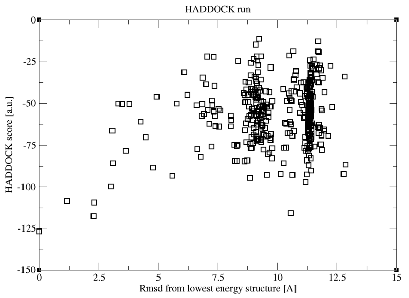
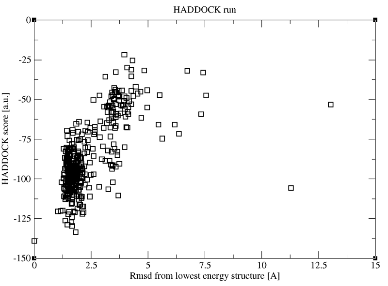
The first and second arguments are the column numbers and the last the data file to use. In the above example we will be plotting the HADDOCK score versus the RMSD from the best scoring model.
The resulting file is called ene_rmsd.xmgr and can be visualized with xmgrace if installed:
The resulting plot shows you a distribution of scores versus the RMSD from the best scoring model.
See plot:
While such plots allow you to visualise the distribution of scores and RMSDs in your ensemble of model, we usually rather cluster the models, and score the resulting clusters, which will be described in the next section.
Cluster-based analysis
One section of run.cns which we have not modified in this example specifies the clustering method and paramters:
{* Clustering method (RMSD or Fraction of Common Contacts (FCC)) *}
{+ choice: "RMSD" "FCC" +}
{===>} clust_meth="FCC";

{* RMSD cutoff for clustering? (Recommended values: RMSD 7.5, FCC 0.60) *}
{===>} clust_cutoff=0.60;

{* Minimum cluster size? *}
{===>} clust_size=4;

{* Chain-Agnostic Algorithm (used for FCC clustering in symmetrical complexes) *}
{+ choice: "true" "false" +}
{===>} fcc_ignc=false;
HADDOCK supports two different clustering methods:
- One is based on the fraction of common contacts between the molecules (FCC clustering) (for details see the online manual)
- One is based on the ligand interface RMSD (here the structures are first fitted on the interface of the first molecule and then the RMSD is calculated on the interface of the remaining molecules (for details see the online manual)
The default is FCC (also recommended for multimeric complexes). For small ligand and peptide docking we however recommend using the RMSD clustering option with reduced cutoffs of 2.0Å and 5.0Å, respectively.
The minimum cluster size is set to 4, but in case the clustering fails, HADDOCK will automatically reduce it.
The clustering output cluster.out can be found in the analysis directories, both in the it1 and water directories. Unzip the file if necessary. For this particular example, its content should look like:
Cluster 1 -> 349 15 17 26 29 32 37 41 46 49 50 52 54 68 69 72 73 74 78 83 88 91 92 94 98 100 101 105 107 110 117 122 124 125 126 128 135 137 139 1
41 145 146 152 153 154 155 157 158 159 161 163 164 167 169 177 182 183 184 185 189 192 193 196 197 200 205 210 211 214 217 219 220 225 227 230 234
 238 247 250 252 253 254 255 256 257 258 260 273 275 277 278 283 284 285 286 290 296 297 298 300 306 309 319 321 323 326 327 330 331 333 335 337 3
39 344 345 348 355 357 358 359 364 366 367 375 377 378 387 388
Cluster 2 -> 320 8 11 21 22 23 24 27 30 31 36 39 40 51 53 55 59 60 61 62 64 65 66 67 70 75 80 81 85 87 89 90 93 99 111 112 114 119 120 127 131 132
 140 142 144 149 150 160 165 168 170 171 172 179 180 181 186 191 198 199 202 206 207 212 218 226 229 231 232 235 237 243 251 272 276 280 289 291 3
04 313 314 318 322 334 343 352 356 362 392
Cluster 3 -> 242 63 82 84 97 116 130 134 162 190 216 267 270 301 312 338 346 347 351 363 380 397
Cluster 4 -> 368 195 203 262 268 299 311 329 350 361 376 382 384 386 389
Cluster 5 -> 294 71 77 178 224 259 279 293 295 305 308 317
Cluster 6 -> 187 28 38 118 121 174 213 240 264 328 342
Cluster 7 -> 310 7 25 79 96 102 138 147 188
Cluster 8 -> 353 47 95 104 109 113 115 340
Cluster 9 -> 315 57 263 303 336
Cluster 10 -> 266 14 20 44 143
Cluster 11 -> 244 48 136 201 204
Cluster 12 -> 194 236 302 324 325
Cluster 13 -> 173 34 58 108
Cluster 14 -> 5 1 2 4
The clusters are sorted and numbered in order of their size. The first number after the arrow corresponds to the cluster center. The number themselves correspond to the ranking of the models in the it1 or water directories. For example, model 15 in this list corresponds to the 15th ranked model in the water directory, corresponding to antibody-antigen_138w.pdb (which can be found in file.nam). The PDB files present in the analysis directory have however been renumbered according to their rank.
We will now perform a cluster-based analysis and ranking, calculating the average score (and other statistics) over each cluster. However to avoid having the size of the cluster affect its score, we rather consider a same number of models for each cluster, e.g. 4 (the minimum number of models defining a cluster). The perform this analysis, type in the water directory the following command:
$HADDOCKTOOLS/ana_clusters.csh -best 4 analysis/cluster.out
This generates a variety of data files, the most interesting one being clusters_haddock-sorted.stats_best4 which lists the various terms following the clusters and their corresponding average score and other energy terms based on their average HADDOCK score. For details refer to the online manual.
#Cluster haddock-score sd rmsd sd rmsd-Emin sd Nstruc Einter sd Enb sd Evdw+0.1Eelec sd Evdw sd Eelec sd Eair sd Ecdih sd Ecoup sd Esani sd Evean
sd Edani sd #AIRviol sd #dihedviol sd #Coupviol sd #Saniviol sd #Veanviol sd #Daniviol sd BSA sd #dH sd #Edesolv sd
file.nam_clust14 -115.743 7.339 1.433 0.946 1.433 0.946 4 -110.79 70.50 -567.22 23.43 -114.59 2.56 -64.30 4.37 -502.92 26.99 456.43 49.82 0.00 0.0
0 0.00 0.00 0.00 0.00 0.00 0.00 0.000 0.000 9.00 0.71 0.00 0.00 0.00 0.00 0.00 0.00 0.00 0.00 0.000 0.000 2021.175 41.803 0.000 0.000 3.495 1.749
file.nam_clust2 -89.292 4.620 1.482 1.014 8.832 0.460 89 -32.63 47.83 -417.01 57.40 -94.60 2.26 -58.78 6.26 -358.23 63.22 384.38 26.04 0.00 0.00 0
.00 0.00 0.00 0.00 0.00 0.00 0.000 0.000 8.25 0.83 0.00 0.00 0.00 0.00 0.00 0.00 0.00 0.00 0.000 0.000 1783.680 115.230 0.000 0.000 2.697 3.510
file.nam_clust1 -85.455 3.444 1.035 0.640 11.362 0.049 128 -47.75 63.27 -463.55 24.95 -91.90 2.15 -50.60 2.81 -412.95 26.82 415.81 77.45 0.00 0.00
 0.00 0.00 0.00 0.00 0.00 0.00 0.000 0.000 9.75 1.48 0.00 0.00 0.00 0.00 0.00 0.00 0.00 0.00 0.000 0.000 1665.472 51.602 0.000 0.000 6.159 2.172
...
The first row indicates the various terms in the file. In this example we can see that the best cluster according to the HADDOCK score is cluster 14 which has only 4 members.
The RMSD from the best scoring model (rmsd-Emin) indicates that this cluster contains it. The first RMSD value reported corresponds to the average pairwise RMSD within the cluster.
When comparing clusters it is also important to consider the standard deviations of the various scores.
Do the clusters satisfy all the restraints we defined?
Between 8 and 9 restraints are violated on average in this example, out of the 28 AIR restraints we defined. Remember that our definition of active residues in the antibody was based on predicted CDR loops and might not be perfect.
In principle you could analyse which restraints are most often violated.
But in this particular example we only performed the clustering since the following settings were defined in run.cns:
* Full or limited analysis of results? *}
{+ choice: "full" "cluster" "none" +}
{===>} runana="cluster";
To perform the full analysis, you would have to empty the analysis directory, change the setting in run.cns to full and restart HADDOCK.
Note that a full analysis can take quite some time, up to a few hours depending on the number of models generated and the size of your complex.
For details about violations analysis, please refer to the online manual.
Comparison with the crystal structure of this antibody-antigen complex
The crystal structure of the complex we just modelled is available from the PDB database (PDB ID 4G6M).
Let’s consider the top model of the top three clusters (#14, #2 and #1) and compare their structure with the crystal structure of this complex.
We will use for that models from the analysis directory since those do contain a chainID which makes the comparison easier
(HADDOCK/CNS internally uses the segID to identify molecules). Using cluster.out identify the model number
which corresponds to the best scoring model for each of those three clusters and load these in PyMol with:
pymol antibody-antigenfit_1.pdb antibody-antigenfit_8.pdb antibody-antigenfit_15.pdb
show cartoon
hide lines
remove resn HOH
Then load the crystal structure:
fetch 4g6m
show cartoon
hide lines
remove resn HOH
util.cbc
Now align all models onto the crystal reference using the antibody as reference for fitting:
Does it actually correspond to the best scored cluster representative?
Congratulations!
You have now completed this tutorial! But if you are curious about the impact of adding a second cross-link restraint on the docking results,
consider repeating the analysis for another run provided with the data you downloaded (antibody-antigen-run-2xl).
See a preview of the results:
The following plot shows the distribution of HADDOCK scores vs RMSD from the top ranked model for a run using two cross-link restraints. Compared to the run we just analysed, the distribution of points is quite different with a much larger population around the best model. This of course does not mean that that model is the correct one per se. Up to you to figure it out...
If you have any questions or suggestions, feel free to contact us via email, or post your question to
our HADDOCK forum hosted by the
![]() Center of Excellence for Computational Biomolecular Research.
Center of Excellence for Computational Biomolecular Research.