

DisVis web server Tutorial
This tutorial consists of the following sections:
- Introduction
- Setup/Requirements
- Inspecting the data
- Accessible interaction space search
- Analysing the results
- Interaction analysis
- Additional challenge
- Final remarks
Introduction
DisVis is a software developed in our lab to visualise and quantify the information content of distance restraints between macromolecular complexes. It is open-source and available for download from our Github repository. To facilitate its use, we have developed a web portal for it.
This tutorial demonstrates the use of the DisVis web server. The server makes use of either local resources on our cluster, using the multi-core version of the software, or GPGPU-accelerated grid resources of the EGI to speed up the calculations. It only requires a web browser to work and benefits from the latest developments in the software based on a stable and tested workflow. Next to providing an automated workflow around DisVis, the web server also summarises the DisVis output highlighting relevant information and providing a first overview of the interaction space between the two molecules with images autogenerated in UCSF Chimera.
The case we will be investigating is the interaction between two proteins of the 26S proteasome of S. pombe, PRE5 (UniProtKB: O14250) and PUP2 (UniProtKB: Q9UT97). For this complex seven experimentally determined cross-links (4 ADH & 3 ZL) are available (Leitner et al., 2014). We added two false positive restraints - it is your task to try to identify these! For this, we use DisVis to try to filter out these false positive restraints while assessing the true interaction space between the two chains. We will then use the interaction analysis feature of DisVis that allows for a more complete analysis of the residues putatively involved in the interaction between the two molecules. To do so, we will extract all accessible residues of the two partners, and give the list of residues to DisVis using its interaction analysis feature. Finally, we will show how the restraints can be provided to HADDOCK in order to model the 3D interaction between the 2 partners.
DisVis and HADDOCK are described in:
-
G.C.P. van Zundert, M. Trellet, J. Schaarschmidt, Z. Kurkcuoglu, M. David, M. Verlato, A. Rosato and A.M.J.J. Bonvin. The DisVis and PowerFit web servers: Explorative and Integrative Modeling of Biomolecular Complexes.. J. Mol. Biol.. 429(3), 399-407 (2016).
-
G.C.P van Zundert and A.M.J.J. Bonvin. DisVis: Quantifying and visualizing accessible interaction space of distance-restrained biomolecular complexes. Bioinformatics 31, 3222-3224 (2015).
-
G.C.P. van Zundert, J.P.G.L.M. Rodrigues, M. Trellet, C. Schmitz, P.L. Kastritis, E. Karaca, A.S.J. Melquiond, M. van Dijk, S.J. de Vries, A.M.J.J. Bonvin. The HADDOCK2.2 webserver: User-friendly integrative modeling of biomolecular complexes. J. Mol. Biol. 428(4), 720-725 (2016).
Throughout the tutorial, coloured text will be used to refer to questions, instructions, and Chimera commands.
This is a question prompt: try answering it! This is an instruction prompt: follow it! This is a Chimera prompt: write this in the Chimera command line prompt!
Setup/Requirements
In order to follow this tutorial you only need a web browser, a text editor, and UCSF Chimera
(freely available for most operating systems) on your computer in order to visualise the input and output data.
Further, the required data to run this tutorial should be downloaded from here.
Once downloaded, make sure to unpack the archive.
Inspecting the data
Let us first inspect the available data, namely the two individual structures as well as the distance restraints we will provide as input.
Using Chimera, we can easily visualise the models and the identified cross-links, by navigating Chimera’s menus or simply entering the corresponding command within the Chimera command-line interface.
For this open the PDB files PRE5.pdb and PUP2.pdb.
UCSF Chimera Menu → File → Open… → Select the file
Repeat this for each file. Chimera will automatically guess their type.
Note: Make sure to load PRE5.pdb first and than PUP2.pdb in order for the subsequent commands
to work on the correct residues!
If you want to use the Chimera command-line instead, you need to first display it:
UCSF Chimera Menu → Tools → General Control → Command Line
and type:
open /path/to/PRE5.pdb open /path/to/PUP2.pdb
From the command-line you can also adjust the view to properly display both structures by entering:
As a first step, we will display and colour all residues involved in a cross-link. You can find the list of cross-links
in the file restraints.txt. The first column indicates the residues of PRE5 and the second column the
residues of PUP2. To colour and display residues in Chimera, enter following commands in the Command Line:
color red #0:27,49,54,55,122,164
show #0:27,49,54,55,122,164
color orange #1:18,49,125,127,128,169,179,188
show #1:18,49,125,127,128,169,179,188
PS: Make sure the identifiers match the models (#0 → PRE5 and #1 → PUP2).
Does the location of the residues already suggest an interface or which residues might be part of the false positive restraints? We will now try to assess the consistency of the restraints with DisVis and figure out which of those restraints might be false positives thanks to an exhaustive analysis of the interaction space between the two molecules.
Accessible interaction space search
DisVis performs a full and systematic 6 dimensional search of the three translational and rotational degrees of freedom to determine the number of complexes consistent with the restraints. It outputs information about the inconsistent/violated restraints and a density map that represents the center-of-mass position of the scanning chain consistent with a given number of restraints at every position in space.
DisVis requires three input files: two high-resolution atomic structures of the biomolecules to be analysed (PRE5.pdb and
PUP2.pdb) and a text file containing the list of distance restraints between the two molecules (restraints.txt).
This is also the minimal required input for the web server in order to setup a run.
To run DisVis, go to
https://wenmr.science.uu.nl/disvis
On this page, you will find the most relevant information about the server as well as the links to the local and grid versions of the portal’s submission page.
Step1: Register to the server
Register for getting access to the web server (or use the credentials provided in case of a workshop).
You can click on the “Register” menu from any DisVis page and fill the required information. Registration is not automatic but is usually processed within 12h, so be patient.
Step2: Define the input files and parameters and submit
Click on the “Submit” menu to access the input form.
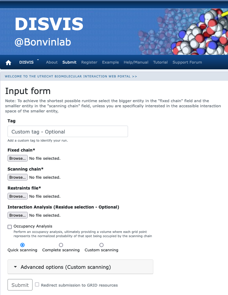
Fixed chain → PRE5.pdb Scanning chain → PUP2.pdb Restraints file → restraints.txt
Once the fields have been filled in, you can submit your job to our server by clicking on “Submit” at the bottom of the page.
If the input fields have been correctly filled you should be redirected to a status page displaying a message indicating that your run has been successfully submitted. While performing the search, the DisVis web server will update you on the progress of the job by reloading the status page every 30 seconds. The runtime of this example case is below 5 minutes on our local CPU and grid GPU servers. However the load of the server as well as pre- and post-processing steps might substantially increase the time until the results are available.
While the calculations are running, open a second tab and go to
https://wenmr.science.uu.nl/disvis
Then click on the “Help/Manual” menu.
Here, you can have a look at the several features and options of DisVis and read about the meaning of the various input parameters (including the ones in “Advanced options”). You can also go back to the submission page and play with the different parameters.
The rotational sampling interval option is given in
degrees and defines how tightly the three rotational degrees of freedom will be
sampled. Voxel spacing is the size of the grid’s voxels that will be cross-correlated during the 3D translational search.
Lower values of both parameters will cause DisVis to perform a finer search, at the
expense of increased computational time. The default values are 15° and 2.0Å for a quick scanning and 9.72° and 1.0Å
for a more thorough scanning.
For the sake of time in this tutorial, we will keep the sampling interval to the quick scanning settings (15.00° and 2.0Å).
The number of processors used for the calculation is fixed to 8 processors on the web server side.
This number can of course be changed when using the local version of DisVis.
Analysing the results
Web server output
Once your job has completed, and provided you did not close the status page, you will be automatically redirected to the results page (you will also receive an email notification).
If you don’t’ want to wait for your run to complete, you can access the precalculated results of a run submitted with the same input here.
The results page presents a summary split into several sections:
Status: In this section you will find a link from which you can download the output data as well as some information about how to cite the use of the portal.Accessible Interaction Space: Here, images of the fixed chain together with the accessible interaction space, in a density map representation, are displayed. Different views of the molecular scene can be chosen by clicking on the right or left part of the image frame. Each set of images matches a specific level of N restraints which corresponds to the accessible interaction space by complexes consistent with at least N restraints. A slider below the image container allows you to change the the number of restraints N and load the corresponding set of images.Accessible Complexes: Summary of the statistics for number of complexes consistent with at least N number of restraints. The statistics are displayed for the N levels, N being the total number of restraints provided in the restraints file (hererestraints.txt)z-Score: For each restraint provided as input, a z-Score is provided, giving an indication of how likely it is that the restraint is a false positive. The higher the score, the more likely it is that a restraint might be a false positive. Putative false positive restraints are only highlighted if no single solution was found to be consistent with the total number of restraints provided. If DisVis finds complexes consistent with all restraints, the z-Scores are still displayed, but should be ignored.Violations: The table in this sections shows how often a specific restraint is violated for all models consistent with a given number of restraints. The higher the violation fraction of a specific restraint, the more likely it is to be a false positive. Column 1 shows the number of consistent restraints N, while each following column indicates the violation fractions of a specific restraint for complexes consistent with at least N restraints. Each row thus represents the fraction of all complexes consistent with at least N restraints that violated a particular restraint. As for the z-Scores, if solutions have been found that are consistent with all restraints provided, this table should be ignored.
It is possible to extract significant results from the results page of this initial run.
As mentioned above, the two last sections feature a table that highlights putative false positive restraints based on their z-Score and their violation frequency for a specific number of restraints. We will naturally look for the crosslinks with the highest number of violations. The DisVis web server preformats the results in a way that false positive restraints are highlighted and can be spotted at a glance.
In our case, you should observe that DisVis found solutions consistent with up to 6 restraints indicating that there might be three false positive restraints.Taking a closer look at the violations table might already be enough to determine which residues are most likely True false positives. In this example two restraints are violated in all complexes consistent with 6 restrains and are thus the most likely candidates:
See solution:
When DisVis fails to identify complexes consistent with all provided restraints during quick scanning it is advisable to rerun with the complete scanning parameters before remove all restraints (or remove only the most violated ones and rerun with complete scanning). It is possible that a more thourough sampling of the interaction space will yield complexes consistent with all restraints or at least reduce the list of putative false positive restraints.
DisVis output files
It is difficult to really appreciate the accessible interaction space between the two partners with only images. Therefore download the results archive to your computer which is available at the top of your results page. You will find in it the following files:
accessible_complexes.out: A text file containing the number of complexes consistent with a number of restraints.accessible_interaction_space.mrc: A density file in MRC format. The density represents the center of mass of the scanning chain conforming to the maximum number of consistent restraints at every position in spacedisvis.log: A log file showing all the parameters used, together with date and time indications.violations.out: A text file showing how often a specific restraint is violated for each number of consistent restraints.z-score.out: A text file giving the Z-score for each restraint. The higher the score, the more likely the restraint is a false positive.run_parameters.json: A text file containing the parameters of your run.result.html: A reduced version of the results page for viewing the results offline or after the data have been deleted from our servers.
Let us now inspect the solutions in Chimera:
Open the fixed_chain.pdb file and the accessible_interaction_space.mrc density map in Chimera.
Use for this either the Menus or the Command-line interface as explained before.
The values of the accessible_interaction_space.mrc slider bar correspond to the number of satisfied restraints (N).
In this way, you can selectively visualise regions where complexes have been found to be consistent with a given number of
restraints. Try to change the level in the “Volume Viewer” to see how the addition of restraints reduces
the accessible interaction space.
How many restraints do you need to significantly reduce the AIS? Can you explain why?
See solution:
The most significant difference can be seen when going from 4 to 5 restraints. By looking closer at the restraints, we can see that two clusters of 3 and 4 residues exist. Once we add a fifth restraint, links from both clusters need to be fulfilled. Thus, significantly reducing the accessible interaction space.
Interaction analysis
We now have an idea of the accessible interaction space between the two molecules defined by the distance restraints.
We can however go further and try to identify what are the most important residues involved in this interaction. This information
might be useful to complement the distance restraints, for example in a docking run to model the complex.
To do so, we will use the Interaction Analysis feature of DisVis. By providing a list of residues, DisVis will analyse which ones
are most contacted in the solutions consistent with the provided distance restraints.
Go to:
https://wenmr.science.uu.nl/disvis/submit
We will use the same input as for the first run of DisVis, but removing this time the false positive
crosslinks identified at the previous step. The new set of restraints can be found in
restraints_filtered.txt:
Fixed chain → PRE5.pdb Scanning chain → PUP2.pdb Restraints file → restraints_filtered.txt
But, in addition, we will now provide a list of residues for the fixed and scanning chains.
These are defined in the text file accessible_res_70.listprovided with the tutorial data.
The residues we have selected are all residues considered as surface accessible for both the fixed
and the scanning chain. We used NACCESS to compute the
solvent accessibility of each residue and selected the accessible ones using a threshold of 40% relative
accessibility for either the backbone or the side-chain.
Interaction Analysis → accessible_res_70.list
For this specific run, we will use the Complete scanning option. By default the server activates
the Occupancy Analysis option when Complete scanning is selected but we will disable it to
keep the computation time in a reasonable window for this tutorial (The occupancy analysis option was enabed in the run on the
Tutorial page so you can access the resulting files by Downloading the associated results archive ).
Select the Complete Scanning radio button Uncheck the Occupancy Analysis checkbox
Expand the Advanced Options group to verify that the sampling interval has been set to 9.72° and 1.0Å.
Then click on the Submit button to start the run.
Once your job has completed, the results page will be displayed. If you don’t want to wait for your run to complete, you can see the results of a pre-calculated run here.
Did the number of satisfied restraints change in comparison to the first quick scanning run?
Next to the previously described sections, it now contains a new section:
Interaction analysis: The tables of this section show how many interactions a specific residue makes in the complexes consistent with a specific number of restraints. The higher the interaction fraction of a specific residue is, the more likely it is to be part of the interface of the complex.
Thanks to this new information, we can now identify putative key residues that should be part of the interface of the complex. The tables can be sorted by their average number of interactions, which allows easy identification of the the most important ones. Depending on the downstream utilization you might be interested in all residues potentially involved in the interaction or a few of the most likely ones. In this specific example considering residues with more than 0.5 interaction on average in the complexes that comply with the maximum number of restraints, results in a reasonable list of residues to e. g. drive the docking of both partners in a HADDOCK docking run.
Note that in the context of using this information to drive the docking in HADDOCK, it is better to be too generous in the definition of the interface rather than too restrictive. Better results are expected if the “true” interface is properly covered. False predictions will not hurt the performance too much since by default HADDOCK will randomly delete for each model a fraction of the provided data.
How many key residues meeting the above mentioned criteria can you identify from the tables? Create a list of these residues for both the fixed and the scanning chain.
See solution:
Respectively 11 and 8 residues have been identified as important for the interaction between PRE5 and PUP2:
PRE5 active residues: 7, 10, 13, 15, 55, 58, 60, 82, 83, 125, 126, 127, 128, 129, 131, 133
PUP2 active residues: 1, 2, 3, 5, 8, 11, 13, 15, 16, 17, 114, 121, 122, 123, 124, 140, 152, 154, 177
You can see the results here
In order to check if those residues are indeed important for the interaction, we will highlight them in Chimera and use a
recently published article (November 2016) structure of a homologue
of the 26S proteasome (from S. cerevisiae). This structure has been solved by X-ray crystallography at 2.4Å resolution (PDBid
5L5A). We will only use the two chains that are of interest,
chains D and C corresponding to PRE5 and PUP2 respectively, in PDB file 5l5a_CD.pdb.
Chimera includes a tool to superimpose structures, allowing us to place our two partners onto the conformation extracted from the S. cerevisiae 26S proteasome.
Re-open a new Chimera session and load the PRE5.pdb, PUP2.pdb and 5l5a_CD.pdb as explained previously.
open /path/to/PRE5.pdb open /path/to/PUP2.pdb open /path/to/5l5a_CD.pdb
Make the main display window active by clicking on it,
Go to Tools → Structure Comparison → MatchMaker In the newly opened MatchMaker window, check “Specific chain in reference structure with best-aligning chain in match structure” in the “Chain Pairing” box.
To superimpose PRE5, do the following:
In the “Reference chain”, select “5l5a_CD.pdb (#2) chain D” and in “Structure(s) to match” select “PRE5.pdb (#0)”. Press Apply to start the optimisation.
What is the RMSD (Root Mean Square Deviation) between PRE5 and chain D of 5L5A (in Å)?
To superimpose PUP2, we will repeat the previous steps:
In the “Reference chain”, select “5l5a_CD.pdb (#2) chain C” and in “Structure(s) to match” select “PUP2.pdb (#1)”. Press Apply to start the optimisation.
What is the RMSD (Root Mean Square Deviation) between PUP2 and the chain C of 5L5A (in Å)?
We can see that S. pombe PRE5 and PUP2 monomers are quite close from the respective homologues in S. cerevisiae.
To ease the subsequent visualisation steps we will first hide the homologous structure 5l5a_CD.pdb.
Go to Favorites → Model Panel Select “5l5a_CD.pdb” and click “hide” on the right panel
In a first step we will visualise the cross-links. This can be done by
drawing a line for each link identified between the corresponding residues.
We can again look at the file gathering the distance restraints to extract the information (restraints.txt).
To draw a line between two atoms in Chimera, we will use the ‘distance’ function. To help you with the atom selection syntax, you can have a look at the ‘atom specification’ section of the Chimera documentation. Here are the commands you need to execute in order to draw all restraints:
distance #0:27@CA | #1:18@CA distance #0:122@CA | #1:125@CA distance #0:122@CA | #1:127@CA distance #0:122@CA | #1:128@CA distance #0:164@CA | #1:49@CA distance #0:55@CA | #1:169@CA distance #0:55@CA | #1:179@CA distance #0:54@CA | #1:179@CA distance #0:49@CA | #1:188@CA
Each restraint present in the restraints.txt file should now be displayed in Chimera. For a better view of these restraints,
you can open the Distances window:
UCSF Chimera Menu → Tools → Structure Analysis → Distances
And now change the Line width, the Line style or even the Color of the distance representations.
Now, we will determine whether the residues identified as active in our last DisVis run are coherent with the conformation of the complex extracted from S.cerevisiae.
First select and colour the key residues identified by DisVis:
color red #0:7,10,13,15,55,58,60,82,83,125,126,127,128,129,131,133 color orange #1:1,2,3,5,8,11,13,15,16,17,114,121,122,123,124,140,152,154,177 show #0:7,10,13,15,55,58,60,82,83,125,126,127,128,129,131,133 show #1:1,2,3,5,8,11,13,15,16,17,114,121,122,123,124,140,152,154,177
See solution:
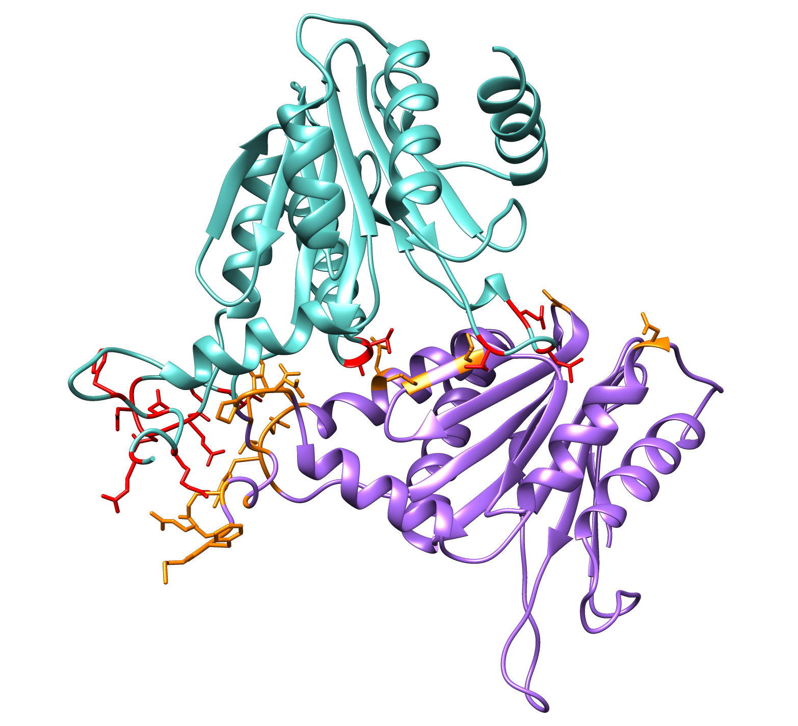
Are the residues given by DisVis consistent with the putative complex of PRE5 and PUP2?
Additional challenge
If time permits try to superpose the reference structure on the fixed chain (PRE5.pdb) and load the accessible interaction space.
You can even rerun DisVis with the occupancy analysis option enabled and repeat the exercise with the generated occupacy_N.mrc files.
Final remarks
We have demonstrated in this tutorial how to make use of the DisVis web server to:
- Identify false positive restraints among a list of restraints obtained either experimentally or via bioinformatic methods and
- Identify key residues involved in the interaction among a list of accessible residues from the two partners.
One should keep in mind that false positive restraints highlighted by DisVis do not necessarily mean wrong restraints. It is also possible that they reflect another binding site of the partners or another conformation of the complex. The identification of different sets of restraints is possible with DisVis but it requires an iterative process in which you will have to test different combinations of restraints.
As we have seen in the last section, one of the limitation of DisVis for identifying key interacting residues is the lack of structural information in the output. DisVis can be a very powerful and accurate to identify key residues involved in the interaction between two partners but it will not provide any contact information. However, this is a very important first step for the purpose of generating a proper model of a complex. Our docking program, HADDOCK, also available as a web server, can, for instance, take key residues identified by DisVis as input (defined as active in HADDOCK) to drive the docking, together with the original distance restraints, in order to generate a biologically relevant model of your complex. Several tutorials describing the use of HADDOCK are available from our tutorial web page. A basic introduction explaining how to define key residues and setup a docking run in HADDOCK is provided in the following tutorial.
Thank you for following this tutorial. If you have any questions or suggestions, feel free to contact us via email, or post your question to
our DisVis forum hosted by the ![]() center of excellence
for computational biomolecular research.
center of excellence
for computational biomolecular research.