HADDOCK2.4 tutorial for the use of template-derived pairwise distance restraints to guide docking

This tutorial consists of the following sections:

• Introduction
• Setup/Requirements
• PS-HomPPI general concepts
• HADDOCK general concepts
• Data for this tutorial
• Running PS-HomPPI to derive CA-CA distance restraints from structural templates
  • Submitting the query to PS-HomPPI
  • Inspecting the PS-HomPPI results
  • Visualizing the CA-CA distance restraints on the structural templates
• CA-CA distance restraint-driven docking with HADDOCK
  • Setting up the docking
    • Registration / Login
    • Submission and validation of structures
    • Definition of restraints
    • Job submission
  • First analysis of the docking results
• Comparison with models obtained by simple superimposition
  • Visualization and comparison of single chain RMSDs
  • Quantitative analysis by l-RMSDs (ligand RMSD) calculation
  • Clash analysis
• Additional/optional questions
• Conclusions
• Congratulations!

Introduction

Although many advanced and sophisticated ab initio approaches for modeling protein-protein complexes have been proposed in past decades, template-based modeling remains the most accurate and widely used approach, provided a reliable template is available. This tutorial will demonstrate the use of HADDOCK for modelling the 3D structure of a protein-protein complex from pairwise interfacial residue distances derived from multiple structural templates.

The case we will be investigating is the complex between bonvine chymotrypsinogen*A and a recombinant variant of human pancreatic secretory trypsin inhibitor (PDB ID: 1ACB). This is one of the cases in the Docking Benchmark 5.0 (BM5), classified as difficult due to the large conformational changes taking place upon binding: The RMSD of CA atoms of interface residues calculated after superposition of bound and unbound interfaces is 2.26Å, and the change in accessible surface area upon complex formation is 1544 Ų.

For this tutorial we will make use the following web servers:

• PS-HomPPI v2.0: A partner-specific homology based protein-protein interface predictor. We use PS-HomPPI to search structural templates from the PDB databank, cluster them and calculate one set of distance restraints from the interfaces of each template cluster.

• HADDOCK2.4: The HADDOCK web portal which allows to model 3D structures of the query complex using distance restraints derived by PS-HomPPI v2.0 to guide the docking.

• R.V. Honorato, M.E. Trellet, B. Jiménez-García1, J.J. Schaarschmidt, M. Giulini, V. Reys, P.I. Koukos, J.P.G.L.M. Rodrigues, E. Karaca, G.C.P. van Zundert, J. Roel-Touris, C.W. van Noort, Z. Jandová, A.S.J. Melquiond and A.M.J.J. Bonvin. The HADDOCK2.4 web server: A leap forward in integrative modelling of biomolecular complexes. Nature Prot., Advanced Online Publication DOI: 10.1038/s41596-024-01011-0 (2024).

A description of the template-based modelling procedure described in this tutorial can be found in the following publication:

• Li C Xue, João P G L M Rodrigues, Drena Dobbs, Vasant Honavar, Alexandre M J J Bonvin. Template-based protein–protein docking exploiting pairwise interfacial residue restraints. Briefings in bioinformatics 18, 458-466 (2017).

Throughout the tutorial, colored text will be used to refer to questions or instructions, and/or PyMOL commands.

This is a question prompt: try answering it! This an instruction prompt: follow it! This is a PyMOL prompt: write this in the PyMOL command line prompt! This is a Linux prompt: insert the commands in the terminal!

Setup/Requirements

In order to follow this tutorial you only need a web browser, a text editor, and PyMOL (freely available for most operating systems) on your computer in order to visualize the input and output data.

PS-HomPPI general concepts

Reliably identifying interfacial residues for protein-protein interactions can provide fundamental insight on protein recognition mechanisms and aid rational drug design. Template-based interface prediction methods are among the most reliable methods. Although many proteins interact with high specificity, the majority of the template-based methods failed to consider interaction partner information.

PS-HomPPI v2.0 is a partner-specific structural template based interface predictor. It is a member of HomPPI, a suite of homology-based interface predictors: 1) NPS-HomPPI (Non partner-specific HomPPI), which can be used to predict interface residues of a query protein in the absence of knowledge of the interaction partner; and (ii) PS-HomPPI (Partner-specific HomPPI), which can be used to predict the interface residues of a query protein with a specific target protein.

PS-HomPPI v2.0 is an improved version of PS-HomPPI v1.3, which has been used to predict pairwise contacts, to reliably rank docked models and to guide flexible docking. However, the major limiting factor for all the template-based methods (including PS-HomPPI) is the availability of the templates. To increase the sensitivity of the PS-HomPPI v1.3 web server, we replaced the BLAST homology search with a Hidden Markov Model based search tool, the HH-suite. Additionally, reliably scoring available templates based on their alignments to the query is also an important factor for the prediction accuracy. To improve this part, v2.0 replaced the multiple linear regression (MLR) model used in v1.3 with a random forest (RF) model for the scoring of the templates. PS-HomPPI v2.0 1) improves the sensitivity of PS-HomPPI, in particular for remote templates, and 2) the RF model provides a more reliable scoring.

PS-HomPPI v2.0 makes pairwise interface predictions with the following steps:

• 1. Search for structural templates. Given queries A and B (assuming A and B interact with each other), PS-HomPPI v2.0 searches the PDB database for structural homologs (as templates) using hhpred.
• 2. Score each templates and select those with highest assigned ranks for predicting the interface of the query. The resulting candidate templates are ranked by a RF-based template scroing function based on the similarity (i.e., hhpred alignment qualities) between the query proteins and the templates. Based on the RF score, each template is assigned as a Safe zone, Twilight Zone 1, Twilight zone 2, or Dark zone template with decreasing interface prediction confidence. If at least one template in the Safe Zone is found, PS-HomPPI uses the Safe homolog(s) to infer the interfaces of the query protein. Otherwise, the process is repeated to use homologs in the Twilight Zone 1, Twilight Zone 2 or the Dark Zone. If no homologs of the query protein can be identified in any of the four defined zones, PS-HomPPI does not provide any predictions.
• 3. Cluster the templates and predict pairwise interfical residues and their distances. To identify different binding modes, the selected templates will be clustered based on the structural similarity. From each cluster, the interfacial residues of the template(s) will be mapped onto the query sequences or structures and the distance distribution of the interfacial residue pairs are calculated using the (multiple) template(s) of this cluster. PS-HomPPI v2.0 reports min, max and average of the distances for each interfacial residue pair.

HADDOCK general concepts

HADDOCK (see https://www.bonvinlab.org/software/haddock2.2) is a collection of python scripts derived from ARIA (https://aria.pasteur.fr) that harness the power of CNS (Crystallography and NMR System – https://cns-online.org) for structure calculation of molecular complexes. What distinguishes HADDOCK from other docking software is its ability, inherited from CNS, to incorporate experimental data as restraints and use these to guide the docking process alongside traditional energetics and shape complementarity. Moreover, the intimate coupling with CNS endows HADDOCK with the ability to actually produce models of sufficient quality to be archived in the Protein Data Bank.

A central aspect to HADDOCK is the definition of Ambiguous Interaction Restraints or AIRs. These allow the translation of raw data such as NMR chemical shift perturbation or mutagenesis experiments into distance restraints that are incorporated in the energy function used in the calculations. AIRs are defined through a list of residues that fall under two categories: active and passive. Generally, active residues are those of central importance for the interaction, such as residues whose knockouts abolish the interaction or those where the chemical shift perturbation is higher. Throughout the simulation, these active residues are restrained to be part of the interface, if possible, otherwise incurring in a scoring penalty. Passive residues are those that contribute for the interaction, but are deemed of less importance. If such a residue does not belong in the interface there is no scoring penalty. Hence, a careful selection of which residues are active and which are passive is critical for the success of the docking.

The docking protocol of HADDOCK was designed so that the molecules experience varying degrees of flexibility and different chemical environments, and it can be divided in three different stages, each with a defined goal and characteristics:

• 1. Randomization of orientations and rigid-body minimization (it0)
  In this initial stage, the interacting partners are treated as rigid bodies, meaning that all geometrical parameters such as bonds lengths, bond angles, and dihedral angles are frozen. The partners are separated in space and rotated randomly about their centers of mass. This is followed by a rigid body energy minimization step, where the partners are allowed to rotate and translate to optimize the interaction. The role of AIRs in this stage is of particular importance. Since they are included in the energy function being minimized, the resulting complexes will be biased towards them. For example, defining a very strict set of AIRs leads to a very narrow sampling of the conformational space, meaning that the generated poses will be very similar. Conversely, very sparse restraints (e.g. the entire surface of a partner) will result in very different solutions, displaying greater variability in the region of binding.

• 2. Semi-flexible simulated annealing in torsion angle space (it1)
  The second stage of the docking protocol introduces flexibility to the interacting partners through a three-step molecular dynamics-based refinement in order to optimize interface packing. It is worth noting that flexibility in torsion angle space means that bond lengths and angles are still frozen. The interacting partners are first kept rigid and only their orientations are optimized. Flexibility is then introduced in the interface, which is automatically defined based on an analysis of intermolecular contacts within a 5Å cut-off. This allows different binding poses coming from it0 to have different flexible regions defined. Residues belonging to this interface region are then allowed to move their side-chains in a second refinement step. Finally, both backbone and side-chains of the flexible interface are granted freedom. The AIRs again play an important role at this stage since they might drive conformational changes.

• 3. Refinement in Cartesian space with explicit solvent (water)
  The final stage of the docking protocol immerses the complex in a solvent shell so as to improve the energetics of the interaction. HADDOCK currently supports water (TIP3P model) and DMSO environments. The latter can be used as a membrane mimic. In this short explicit solvent refinement the models are subjected to a short molecular dynamics simulation at 300K, with position restraints on the non-interface heavy atoms. These restraints are later relaxed to allow all side chains to be optimized.

The performance of this protocol of course depends on the number of models generated at each step. Few models are less probable to capture the correct binding pose, while an exaggerated number will become computationally unreasonable. The standard HADDOCK protocol generates 1000 models in the rigid body minimization stage, and then refines the best 200 – regarding the energy function - in both it1 and water. Note, however, that while 1000 models are generated by default in it0, they are the result of five minimization trials and for each of these the 180º symmetrical solution is also sampled. Effectively, the 1000 models written to disk are thus the results of the sampling of 10.000 docking solutions.

The final models are automatically clustered based on a specific similarity measure - either the positional interface ligand RMSD (il-RMSD) that captures conformational changes about the interface by fitting on the interface of the receptor (the first molecule) and calculating the RMSDs on the interface of the smaller partner, or the fraction of common contacts (current default) that measures the similarity of the intermolecular contacts. For RMSD clustering, the interface used in the calculation is automatically defined based on an analysis of all contacts made in all models.

Data for this tutorial

Data for this tutorial can be downloaded from here. The zipped archive 1ACB.zip contains the INPUT data to run PS-HomPPI and HADDOCK, and pre-calculated PS-HomPPI and HADDOCK outputs. Unzipping this file will create a 1ACB directory containing the following sub-directories and files:

1. INPUT data to PS-HomPPI v2.0 (under 1ACB/PSHomPPI/input):
   • The full sequences of the two individual proteins (query-fasta.txt)
   • A zip file (queryPDBs.zip) containing the PDB files of the two unbound proteins (A.pdb and B.pdb`)
   • The deletion file, which allows users to exclude some specific structural templates (delete.txt). In this case we want to exclude the 1ACB entry since it is the solution to this tutorial.
2. INPUT data to HADDOCK (under 1ACB/HADDOCK/input):
   • CA-CA distance restraints file (cluster1_restraints.tbl). Theses are the ones generated by PS-HomPPI that will be used as input of HADDOCK to guide the docking.
   • The unbound structures of the two individual proteins (A.pdb, B.pdb)
   • The reference PDB file of the complex (1ACB_target.pdb)
   • A reference haddockparam.web file that contains all the input data and settings to run the docking using the File upload interface of the HADDOCK web server.
3. OUTPUT data from PS-HomPPI and HADDOCK (under 1ACB/PSHomPPI/output and 1ACB/HADDOCK/output)
   • Predicted pairwise interfacial residues (CA-CA distances) by PS-HomPPI
   • HADDOCK result page

Note: For facilitating the analysis, the provided unbound and bound structures have been matched, meaning by that that they share the same chain IDs and residue numbering.

Running PS-HomPPI to derive CA-CA distance restraints from structural templates

We will start by using PS-HomPPI v2.0 to

1. search for structural templates,
2. cluster them,
3. and derive interfacial CA-CA distance restraints from each cluster of templates.

Submitting the query to PS-HomPPI

Connect to the the PS-HomPPI web server.

http://ailab-projects2.ist.psu.edu/PSHOMPPIv2.0/

• Step1: Enter your email and give a name to the job

• Step2: Paste the list of query pairs:

Paste a list query ID pairs -> A:B

• Step3: Paste the query protein sequences in fasta format, use for that the content of the querySEQs.fasta.txt file provided in the input folder for PSHomPPI

>A
CGVPAIQPVLSGLSRIVNGEEAVPGSWPWQVSLQDKTGFHFCGGSLINENWVVTAAHCGVTTSDVVVAGEFDQGSSSEKI
QKLKIAKVFKNSKYNSLTINNDITLLKLSTAASFSQTVSAVCLPSASDDFAAGTTCVTTGWGLTRYTNANTPDRLQQASL
PLLSNTNCKKYWGTKIKDAMICAGASGVSSCMGDSGGPLVCKKNGAWTLVGIVSWGSSTCSTSTPGVYARVTALVNWVQQ
TLAAN
>B
TEFGSELKSFPEVVGKTVDQAREYFTLHYPQYDVYFLPEGSPVTLDLRYNRVRVFYNPGTNVVNHVPHVG

• Step4: Upload the PDB files of the query proteins, use for that the queryPDBs.zip file provided in the input folder for PSHomPPI:

Upload PDB files of query proteins in *.tar.gz OR *.zip (recommended) -> queryPDBs.zip

Note: The structures of the individual proteins are optional but recommended. It helps PS-HomPPI 1) to better align the template structures to the query structures, hence more accurate CA-CA distance restraints, and 2) to map the CA-CA distance restraints to the residue numbering of the query proteins. In other words, if the query protein structures are not provided to PS-HomPPI, the output CA-CA distance restraints need to be renumbered according to the query PDB files in order to be used by HADDOCK in the next step.

• Step5: To objectively evaluate the performance of PS-HomPPI, we should exclude the reference complex 1ACB as a possible template. For this we should create a deletion file (delete.txt), in which we specify that we want to exclude our target 1ACB from being used by PS-HomPPI when making interface predictions. For convience this file has already been created and can be found in the PSHomPPI/input folder.

Paste the deletion file (optional) -> A:B=>1acb*

Note: _For more details of the format for the deletion file, see the overview page of the PS-HomPPI 2.0 web server.

• Step6: Define the distance cutoff to create the “CA-CA (Alpha carbon-Alpha carbon) distance restraints. We will leave it to the default of 15 Å.

CA-CA (Alpha carbon-Alpha carbon) distance Threshold -> 15

• Step7: You are ready to submit your job since we will leave all other parameters to their default values.

Click on the submit button!

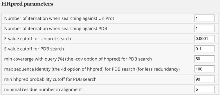
Note: PS-HomPPI v2.0 is powered by the HHpred suite to search for homologs.

See the default HHpred parameters used by PS-HomPPI v2.0

Inspecting the PS-HomPPI results

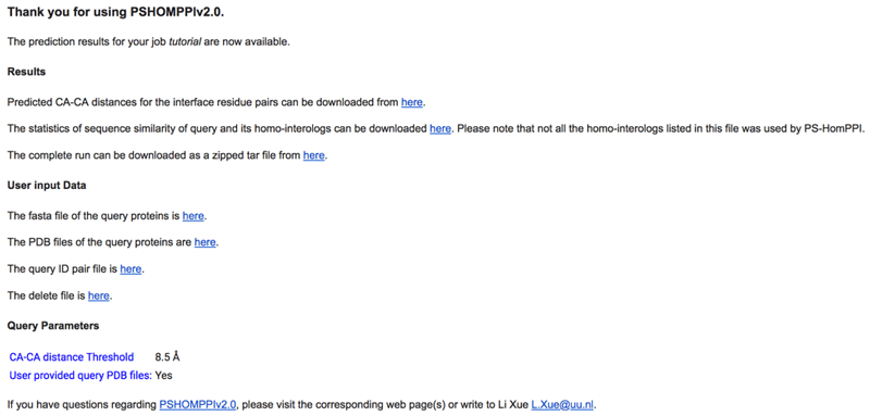
Once finished, PS-HomPPI will send a result email to your email address. It typically takes PS-HomPPI v2.0 about 5-10 minutes for one pair of query proteins.

See an example results email sent by PS-HomPPI v2.0

From links provided in the email, you can download the predicted CA-CA distances for your query proteins A and B (the cluster1_Ca_Ca_distance.txt file). This file is already provided in the tutorial data you downloaded under 1ACB/PSHomPPI/output):

Prediction results of Partner-specific interface residues by PS-HomPPI (http://ailab-projects2.ist.psu.edu/PSHOMPPIv2.0){:target="_blank"}.

Notations:
        1. A|A:B: the interface residues of protein A that interact with protein B.
        2. MODE:
                 Mode = SafeMode: the query protein can find homologous interacting pairs in Safe Zone.
                 Mode = TwilightMode1: the query protein can find homologous interacting pairs in Twilight Zone 1.
                 Mode = TwilightMode2: the query protein can find homologous interacting pairs in Twilight Zone 2.
         For more details about the Safe/Twilight/Dark Zone, please refer to the paper for PS-HomPPI:
        Xue, L. C., Dobbs, D., & Honavar, V. (2011). HomPPI: A Class of sequence homology based protein-protein interface prediction methods. BMC Bioinformatics, 12, 244.
        3. pINT: predicted interface residues. 1: interface. 0: non-interface. ?: no prediction can be made.
        4. SCORE: prediction score from PS-HomPPI. The higher the score the higher prediction confidence.

-----------------------------------------

 Mode = SafeMode
 chnID_Qry1 aa_Qry1 chnID_Qry2 aa_Qry2 mean min max
 A 40 B 51 14.34 14.12 14.83
 A 40 B 45 12.47 12.26 12.69
 A 40 B 49 9.88 9.38 10.57
 A 40 B 70 11.72 11.24 12.14
...
 

Note: If you download a full tar archive from PS-HomPPI, the CA-CA distance files can be found in the following directory: Ca_Ca_distances/A:B (assuming your query proteins were called A and B).

PS-HomPPI v2.0 reports 4 types of prediction confidence based on the sequence similarity between the query proteins and the templates: Safe zone, Twilight zone 1, Twilight zone 2 and Dark zone, ranging from the highest to the lowest confidence levels. For the case in this tutorial, the interface prediction confidence from PS-HomPPI v2.0 is Safe Mode, which indicates the structural templates are quite reliable. This file describes the predicted pairwise CA-CA distances for the predicted interface residues of the query protein pairs. PS-HomPPI v2.0 typically provides multiple CA-CA distance files, one file for one cluster of templates. For this tutorial, only one cluster of templates is identified by PS-HomPPI, hence only one CA-CA distance file is returned: cluster1_Ca_Ca_distance.txt.

In addition to this, PS-HomPPI v2.0 also provides us with distance-restraint files that can be directly used by HADDOCK (the cluster1_restraints.tbl file under the same folder):

! generated by genHaddockRestrFL.pl
! CA-CA cutoff = 15
! 0.5 angstroms are added both sides of the distance restraints derived from templates
assign (name ca and segid A and resi 40) (name ca and segid B and resi 51) 14.340 0.720 0.990
assign (name ca and segid A and resi 40) (name ca and segid B and resi 45) 12.470 0.710 0.720
assign (name ca and segid A and resi 40) (name ca and segid B and resi 49) 9.880 1.000 1.190
...

Distance restraints for use in HADDOCK are defined as (following the CNS syntax):

    assign (selection1) (selection2) distance, lower-bound correction, upper-bound correction

The lower limit for the distance is calculated as: distance minus lower-bound correction, and the upper limit as: distance plus upper-bound correction. There is often confusion about this definition of lower and upper distance bounds, something we addressed in a recent correspondence to Nature Protocols.

Here would be an example of a distance restraint between the alpha carbons (CAs) of residues 128 and 21 in chains A and B with an allowed distance range between 13.263 (= 13.999-0.736) and 14.708 (= 13.999+0.709) Å:

assign (name ca and segid A and resi 128) (name ca and segid B and resi 21) 13.999 0.736 0.709

The distance range is calculated from the standard deviation of the measured distances in all selected templates.

Can you write a new distance restraint for the CA atom of residue 34 in chain A and the CA atom of residue 100 in chain B so that the average distance is 8 Å, and the minimum distance is 6 Å and the maximum distance is 11 Å?

    assign (name ca and segid A and resi 34) (name ca and segid B and resi 100) 8 2 3

You can also inspect the list of templates that have been found bu PS-HomPPI to make the prediction in the templates_used_in_prediction.lst file. This is a simple text file you can inspect using your favoriate text editor, such as vim, TextEdit, Word. In this case, five templates have been used by PS-HomPPI when making the interface predictions:

#Template_ID    predicted_CC
4b2aA,396:4b2aB,7   0.720
4b2aC,396:4b2aD,7   0.720
4h4fA,442:4h4fB,2   0.710
3rdzB,392:3rdzD,58  0.710
3rdzA,392:3rdzC,58  0.710

The column of “Template_ID” indicates the PDB and chain IDs of the selected templates. The integers after the commas are just unique identifiers for the alignments between the query and a template and can be ignored. The column of “predicted_CC” is the prediction confidence of PS-HomPPI v2.0. It ranges from 0 to 1, where 0 is the lowest confidence and 1 the highest confidence.

Visualizing the CA-CA distance restraints on the structural templates

Before we use the CA-CA distances predicted by PS-HomPPI v2.0 to guide docking, let’s visually check these CA-CA distances on structural templates (many times visual check can easily identify wrong CA-CA restraints, if there is any). We are going to use the cluster1_Ca_Ca_distance.pml file generated by PS-HomPPI to do that. This file is actually a PyMol script that will display the distance restraints as dashes between the predicted residue pairs. You can either copy its content and paste it in the top command window of PyMol or execute it directly from within PyMol by typing @cluster1_Ca_Ca_distance.pml in the top command window of PyMol.

The residue numbers in the CA-CA distance restraint files (clusterXX_Ca_Ca_distance.txt and the corresponding xxx.tbl and xxx.pml files) are the same as those in the query PDB files (if they have been uploaded to PS-HomPPI) or the same as the numbering in the query sequences (if no query PDB files were provided). In this tutorial, since we did upload query PDB files, the residue numbering of the distance restraints is the same as the query PDB files. This makes the visualization in PyMol straight-forward.

To visualize the CA-CA distances, let’s use the superimposed models generated by superimposing the individual query structures to the template structures. These superimposed models are automatically generated by PS-HomPPI v2.0. In a downloaded run you wil find them under .../PSHomPPI_results/output/A:B/superimposed_models/supUnbound2TemplatePDB/final/cluster1/finalSup.xxx.pdb (one cluster, one pml file). The corresponding files are also provided in the tutorial data you downloaded under 1ACB/PSHonPPI/output/templates

Check the templates_used_in_prediction.lst file mentioned in the previous section to find out how many templates were selected by PSHomPPI.

4b2aA_4b2aB
4b2aC_4b2aD
4h4fA_4h4fB
3rdzB_3rdzD
3rdzA_3rdzC

Now, let’s visually check the predicted CA-CA restraints on the superimposed selected templates.

Start PyMol and load all PDB files from the 1ACB/PSHonPPI/output/templates directory

Note: If working under Linux or OSX, you can start PyMol with as arguments all PDB filenames in the 1ACB/PSHonPPI/output/templates directory. Alternatively, you can open each file from the File -> Open menu.

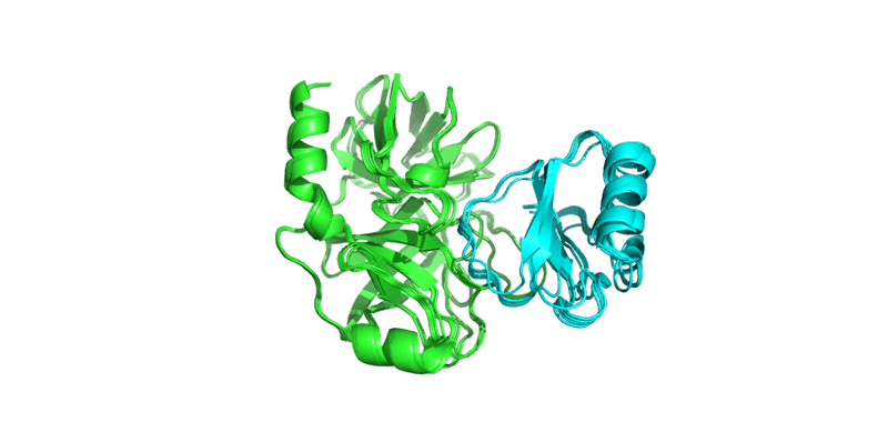
In Pymol, align all superimposed models. Type for this the following command in the Pymol console:

alignto finalSup.3rdzA_3rdzC.template5,
zoom
util.cbc

We can see that the superimposed models in cluster 1 have similar structures, as expected.

Now let’s visualize the CA-CA distance restraints on these models. We will run for the this the PyMol script generated by PS-HomPPI using the File menu:

File -> Run script… -> locate and upload the “cluster1_Ca_Ca_distance.pml” file in the tutorial data folder “1ACB/PSHomPPI/output”

hide labels

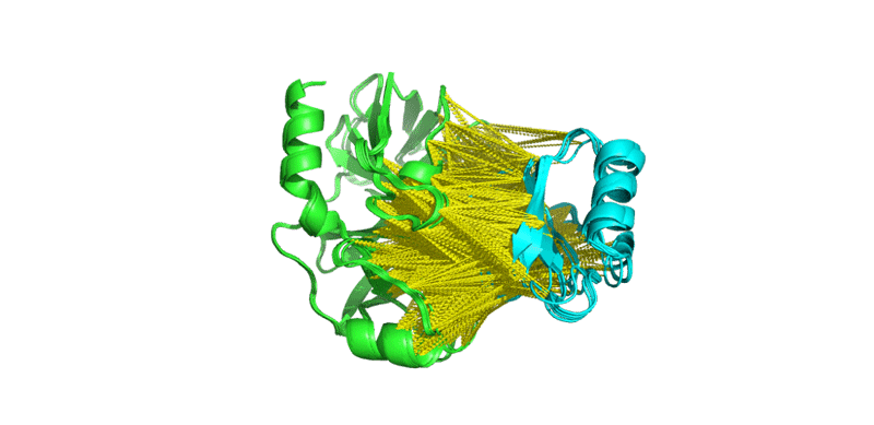
We can see that the CA-CA distance restraints (yellow dashes) are mostly at the interface between the two proteins, hence they seem reasonable. A bad prediction might connect residues that are very remote from the interface. (Remember that the numbering in those models is based on your query PDB files).

CA-CA distance restraint-driven docking with HADDOCK

Setting up the docking

As we have seen in the previous section, PS-HomPPI returns Safe Mode as prediction confidence, which indicates that the structural templates are quite reliable. Therefore, we will use the CA-CA distance restraints as “unambiguous restraints” in HADDOCK (which means that they all will be used during the docking). If you are less confident in the predictions, you might decide to upload the restraints in the ambiguous category. In that case 50% will be randomly deleted for each docking trial.

For CA-CA guided docking, considering our interface prediction are classified as reliable and to save time we can reduce the number of docked models to 50, 50, 50 for the rigid-body, semi-flexible and explicit solvent refinement stages, respectively. To further save running time, the number of trials for rigid body minimization is set to 1 and the sampling of 180 degrees rotated solutions during rigid body EM (Energy Minimization) is turned off.

Registration / Login

In order to start the submission, either click on “here” next to the submission section, or click here. To start the submission process, we are prompted for our login credentials. After successful validation of our credentials we can proceed to the structure upload.

Submission and validation of structures

We have now all the required information to setup our targeted docking run. We will again make use of the HADDOCK2.4 interface, using expert or guru level access (provided with course credentials if given to you, otherwise register to the server and request this access level) here.

Note: The blue bars on the server can be folded/unfolded by clicking on the arrow on the left

• Step1: Define a name for your docking run, e.g. CA-CA-docking.

• Step2: Input the first protein PDB file. For this unfold the First Molecule menu.

First molecule: where is the structure provided? -> “I am submitting it” Which chain to be used? -> All (for this particular case) PDB structure to submit -> Browse and select from the 1ACB/HADDOCK/input directory A.pdb Segment ID to use during docking -> A

• Step3: Input the second protein PDB files. For this unfold the Second Molecule menu.

Second molecule: where is the structure provided? -> “I am submitting it” Which chain to be used? -> All (for this particular case) PDB structure to submit -> Browse and select from the 1ACB/HADDOCK/input directory B.pdb Segment ID to use during docking -> B

• Step 4: Click on the “Next” button at the bottom left of the interface. This will upload the structures to the HADDOCK webserver where they will be processed and validated (checked for formatting errors). The server makes use of Molprobity to check side-chain conformations, eventually swap them (e.g. for asparagines) and define the protonation state of histidine residues.

Definition of restraints

If everything went well, the interface window should have updated itself and it should now show the list of residues for molecules 1 and 2. Instead of specifying active and passive residues, you supply a HADDOCK restraints TBL file (unambiguous restraints). For this click on the “Next” button in the Input parameters window.

• Step5: Input the CA-CA distance restraints from PS-HomPPI. For this unfold the Distance Restraint menu of the Docking Parameters window.

Upload the CA-CA distance restraints file from the 1ACB/HADDOCK/input directory called cluster1_restraints.tbl under the ambiguous distance restraints.

• Step5: Change the sampling parameters to reduce the docking time. For this unfold the Sampling Parameter menu.

Number of structures for rigid body docking _cluster1_restraints.tbl -> 200 Sample 180 degrees rotated solutions during rigid body EM -> Uncheck Refine with short molecular dynamics in explicit solvent? -> Check Number of structures for semi-flexible refinement -> 50 Number of structures for the final refinement -> 50

Job submission

This interface allows us to modify many parameters that control the behaviour of HADDOCK but in our case the default values are all appropriate. It also allows us to download the input structures of the docking run (in the form of a tgz archive) and a haddockparameter file which contains all the settings and input structures for our run (in json format). We strongly recommend to download this file as it will allow you to repeat the run after uploading into the file upload inteface of the HADDOCK webserver. It can serve as input reference for the run. This file can also be edited to change a few parameters for example. An excerpt of this file is shown here:

{
  "runname": "CA-CA-docking",
  "auto_passive_radius": 6.5,
  "create_narestraints": true,
  "delenph": true,
  "ranair": false,
  "cmrest": false,
...

This file contains all parameters and input data of your run, including the uploaded PDB files and the CA-CA restraints.

Can you locate the distance restraints in this file?

• Step 6: You are ready to submit!

Click on the “Submit” button at the bottom left of the interface.

Upon submission you will be presented with a web page which also contains a link to the previously mentioned haddockparameter file as well as some information about the status of the run.

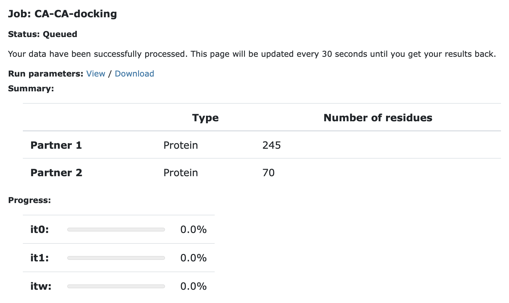
Currently your run should be queued but eventually its status will change to “Running”:

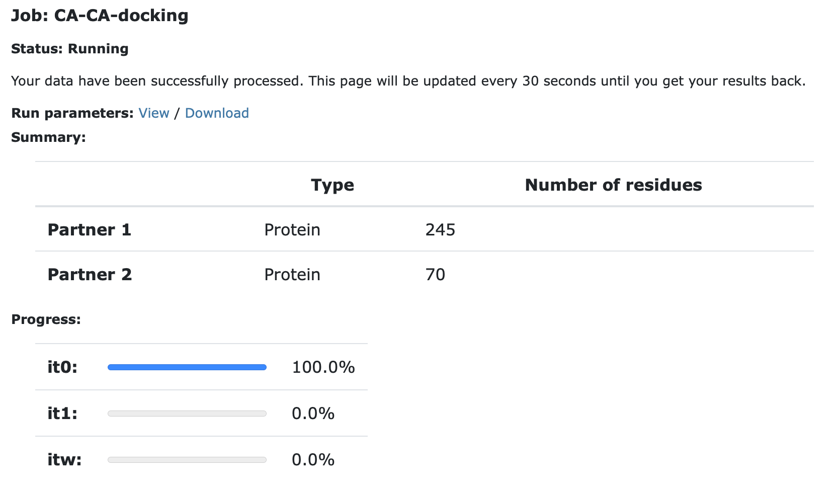
The page will automatically refresh and the results will appear upon completion (which can take between 1/2 hour to several hours depending on the size of your system and the load of the server). You will be notified by email once your job has successfully completed.

First analysis of the docking results

Once your run has completed you will be presented with a result page showing the cluster statistics and some graphical representation of the data (and if registered, you will also be notified by email).

In case you don’t want to wait for your results, you can find it here. The result page should look like:

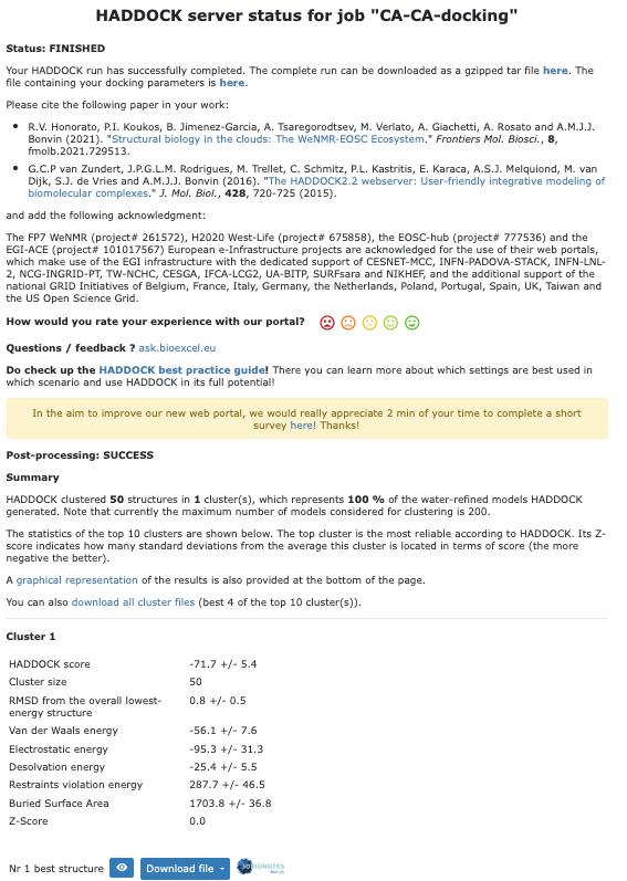
Inspect the result page How many clusters are generated? Is this expected?

Note: The bottom of the page gives you some graphical representations of the results, showing the distribution of the solutions for various measures (HADDOCK score, van der Waals energy, …) as a function of the RMSD from the best generated model (the best scoring model).

The ranking of the clusters is based on the average score of the top 4 members of each cluster. The score is calculated as:

      HADDOCKscore = 1.0 * Evdw + 0.2 * Eelec + 1.0 * Edesol + 0.1 * Eair

where Evdw is the intermolecular van der Waals energy, Eelec the intermolecular electrostatic energy, Edesol represents an empirical desolvation energy term adapted from Fernandez-Recio et al. J. Mol. Biol. 2004, and Eair the AIR energy. The cluster numbering reflects the size of the cluster, with cluster 1 being the most populated cluster. The various components of the HADDOCK score are also reported for each cluster on the results web page.

In this particular case, since we have very specific distance restraints, only one cluster is present.

Let’s now visualize the top 4 models and compare those to the crystal structure of the target structure (PDB ID: 1ACB).

Download and save to disk the top 4 members of the cluster

Then start PyMOL and load each cluster representative:

File menu -> Open -> select cluster1_1.pdb

Repeat this for each model.

In order to check if any of the docking models we obtained makes sense, we will compare them to the experimentally determined target structure (PDB ID: 1ACB). This structure has been solved by X-ray crystallography at 2 Å resolution. We will now download the reference structure directly from the Protein Data Bank. For this type in the PyMol command window:

fetch 1ACB

Note: In PyMol you can toggle on and off models by clicking in the model name in the rigth panel.

Look at the just downloaded 1ACB structure. What are the crosses in the PyMol window?

The downloaded PDB entry has different chain IDs than what we used for the docking. In order to simplify the analysis, we will first rename the chains and also remove all solvent molecules. For this type in the PyMol command window:

alter (chain E and 1ACB), chain="A"
alter (chain I and 1ACB), chain="B"
remove solvent

Let’s now superimpose all docking models onto chain A of the reference complex 1ACB:

select 1ACB_A, 1ACB and chain A
alignto 1ACB_A
zoom
util.cbc
color pink, 1ACB and chain A
color red, 1ACB and chain B

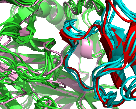
We can see that the docked models (green and blue) have similar interfaces as those in the X-ray structure of the target (pink and red).

Inspect the models and the reference structure Can you locate regions with conformational changes?

See solution:

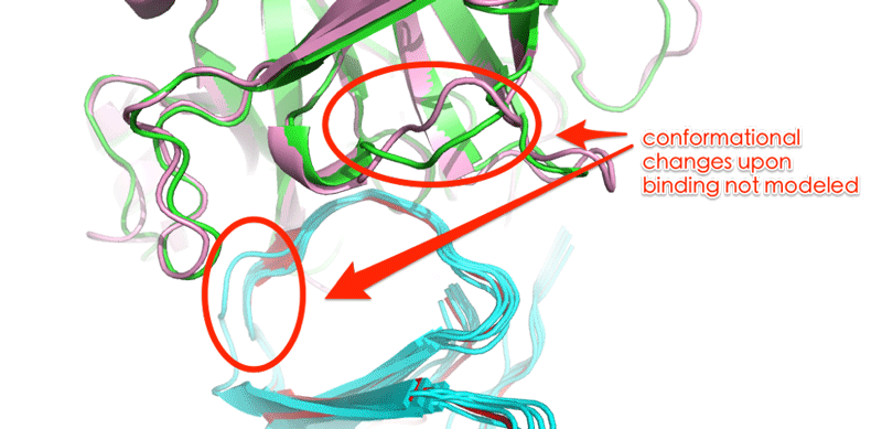
We can see that the superimposed models (green and blue) differ from the target structure (pink and red) at the interface in some loops, failing to model conformational changes upon binding. In our modelling we are limited by the amount of conformational changes HADDOCK can handle, but also but also by the CA-CA distance restraints that are limited to the spread observed in the selected templates. The question is: Are these models better than you would obtain by a simple superimposition, something we will address in the following section.

Note: Keep your PyMol session open since we will need it in the following section (or save it for reuse later). In that way you won’t have to repeat all PyMol commands to visualize and superimposed the CA-CA docked models.

Comparison with models obtained by simple superimposition

Superimposition is one of the simplest and widely used template-based modelling methods. It is based on global structure–structure alignments, and generates models by superimposing unbound 3D component protein (or domain) structures onto structure templates. However, superimposition typically treats individual unbound structures as rigid and thus cannot model any conformational changes occuring upon binding. Further it tends to generate large numbers of steric clashes at the interface, requiring a further refinment step.

In contrast, the CA-CA guided docking protocol treats the interface as flexible since HADDOCK allows for flexibility at the interface during the simulated annealing stage and final refinement in explicit solvent. This allows some optimization of the conformation of the backbone and sidechains of the docked interface. But don’t expect miracles! The amount of conformational changes modelled in that way will still be limited. In Xue et al. 2017, we have shown that our CA-CA guided docking protocol is superior to simple superimposition for cases with medium to large conformations upon binding.

Visualization and comparison of single chain RMSDs

In this section we will compare superimposed models with our CA-CA guided models. PS-HomPPI v2.0 automatically generates superimposed models. These are stored under .../PSHomPPI_results/output/A:B/superimposed_models/supUnbound2TemplatePDB/final/finalSup when downloading the results archive from the server. We are also providing those models directly in the downloaded tutorial data in the 1ACB/PSHomPPI/output/superimposed-models folder.

Load in PyMol all models from the 1ACB/PSHomPPI/output/superimposed-models tutorial data folder

Color them in yellow to better distinguish them and superimpose them as we did before on chain A of the reference complex

color yellow, model*
alignto 1ACB_A
zoom

Inspect the information panel on the top of the window and compare the reported RMSD values of the CA-CA docked models and the superimposed models. These only report on the RMSD to chain A of the reference complex. Which modelling strategy leads to smaller RMSDs?

cluster1_1           RMSD =    1.787 (232 atoms)
cluster1_2           RMSD =    1.785 (232 atoms)
cluster1_3           RMSD =    1.720 (232 atoms)
cluster1_4           RMSD =    1.736 (232 atoms)
1ACB                 RMSD =    0.000 (240 atoms)
model1-4b2aA_4b2aB   RMSD =    1.814 (232 atoms)
model2-4b2aC_4b2aD   RMSD =    1.814 (232 atoms)
model3-4h4fA_4h4fB   RMSD =    1.814 (232 atoms)
model4-3rdzB_3rdzD   RMSD =    1.814 (232 atoms)
model5-3rdzA_3rdzC   RMSD =    1.814 (232 atoms)

Repeat this, but superimposing now on chain B.

select 1ACB_B, 1ACB and chain B
alignto 1ACB_B

Again, which modelling strategy leads to smaller RMSDs? Which of the two chains undergoes larger conformational changes?

cluster1_1           RMSD =    1.142 (56 atoms)
cluster1_2           RMSD =    0.755 (56 atoms)
cluster1_3           RMSD =    1.174 (56 atoms)
cluster1_4           RMSD =    0.782 (56 atoms)
1acb                 RMSD =    0.000 (56 atoms)
model1-4b2aA_4b2aB   RMSD =    1.551 (56 atoms)
model2-4b2aC_4b2aD   RMSD =    1.550 (56 atoms)
model3-4h4fA_4h4fB   RMSD =    1.551 (56 atoms)
model4-3rdzB_3rdzD   RMSD =    1.551 (56 atoms)
model5-3rdzA_3rdzC   RMSD =    1.550 (56 atoms)

Can you see which part of chain B undergoes the largest conformational changes?

See solution:

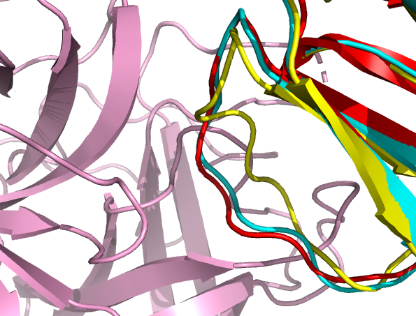
We can clearly see that the inhibitory loop is moving toward the bound conformation. The starting conformation is shown in yellow and the CA-CA docked models in blue. The latter have moved closer to the bound conformation shown in red.

Quantitative analysis by l-RMSDs (ligand RMSD) calculation

In order to have a more quantitative view of the quality of the models we will calculate ligand RMSDs (l-RMSDs). These are used in the blind protein-protein prediction experiment CAPRI (Critical PRediction of Interactions) as a measure of the quality of a model. The l-RMSD is calculated by fitting on the backbone atoms the receptor (first molecule) and calculating the RMSD on the backbone atoms of the ligand (second molecule).

In CAPRI, the l-RMSD value defines the quality of a model:

• acceptable model: l-RMSD<10Å
• medium quality model: l-RMSD<5Å
• high quality model: l-RMSD<1Å

To calculate the l-RMSD of the various models, execute for each model the following commands in PyMol:

align cluster1_1 and chain A and name CA+C+N+O, 1ACB and chain A, cycles=0
rms_cur cluster1_1 and chain B and name CA+C+N+O, 1ACB and chain B, cycles=0

For each model take note of the RMSD value reported after the rms_cur command in the top window.

cluster1_1 -> Executive: RMSD = 1.541 (252 to 252 atoms)
cluster1_2 -> Executive: RMSD = 1.288 (252 to 252 atoms)
cluster1_3 -> Executive: RMSD = 2.130 (252 to 252 atoms)
cluster1_4 -> Executive: RMSD = 1.399 (252 to 252 atoms)

model1-4b2aA_4b2aB -> Executive: RMSD = 2.224 (252 to 252 atoms)
model2-4b2aC_4b2aD -> Executive: RMSD = 1.828 (252 to 252 atoms)
model3-4h4fA_4h4fB -> Executive: RMSD = 3.315 (252 to 252 atoms)
model4-3rdzB_3rdzD -> Executive: RMSD = 1.588 (252 to 252 atoms)
model5-3rdzA_3rdzC -> Executive: RMSD = 1.673 (252 to 252 atoms)

What is the quality of the best model based on te CAPRI l-RMSD criterion ?

By comparing the l-RMSDs of CA-CA models and those of superimposed models, we can see that the CA-CA models have smaller l-RMSDs.

Note: _In CAPRI another measure of quality is also used, the interface RMSD (i-RMSD). It is calculated on the backbone atoms of all residues within 10Å from the the other molecule. It is not possible to calculate i-RMSDs easily in PyMol (we usually use ProFit for this).

Clash analysis

We have previously mentioned the issue of clashes when generating models by simple superimposition. We can check if this is indeed true by running for example a validation server on the models. Here we provide a simple C++ program that calculates the contacts between chains for a given distance cutoff. We can use a 2.5Å cutoff to detect clashes.

Call the contact program located in the 1ACB/scripts directory that was created when you unpacked the downloaded archive (make sure to run first Make in the script directory to compile the program).

<path>/1ACB/scripts/contact-chainID <pdb-file> 2.5 | wc | awk ‘{print $1}’

Let us select the best l-RMSD model from the CA-CA docking and the superimposition (these should be cluster1_2 and model4-3rdzB_3rdzD, respectively).

The reported number of bumps (short contacts <2.5A) are:

• for the CA-CA guided HADDOCK model -> 0
• for the superimposed template -> 72

This clearly demonstrates that the CA-CA docking protocol not only leads to better ligand RMSDs, but also a better quality of the interface. Models obtained by superimposition only need thus to be refined.

Additional/optional questions

1) If you are curious, try refining the superimposed models through it and see if the clashes are removed to the same extend of the CA-CA docked model and if the l-RMSD improves of not. One option to do that is to make use of the HADDOCK2.4 refinement interface available from https://wenmr.science.uu.nl/haddock2.4/refinement/1. Several refinement protocols are provided. For details on their performance refer to our recent Structure paper:

• T Neijenhuis, S.C. van Keulen and A.M.J.J. Bonvin. Interface Refinement of Low-to-Medium Resolution Cryo-EM Complexes using HADDOCK2.4. Structure 30, 476-484 (2022).

2) You could repeat this tutorial changing the “CA-CA (Alpha carbon-Alphacarbon) distance Threshold” parameter of PS-HomPPI v2.0 from 15 Å to 8.5 Å. Check then how this impacts the quality of the docking models.

Conclusions

We have demonstrated the use of CA-CA distance restraints from multiple templates to guide the docking process in HADDOCK. The CA-CA distance restraints were derived from PS-HomPPI v2.0. We have shown that CA-CA guided flexible docking is able to induce conformational changes toward the bound state and further results in good quality models without clashes at the interface, which is clearly not the case for simple superimposition.

Congratulations!

Thank you for following this tutorial. If you have any questions or suggestions, feel free to contact us via email, or post your question to our HADDOCK forum hosted by the Center of Excellence for Computational Biomolecular Research.