

HADDOCK2.4 Antibody - Antigen tutorial using PDB-tools webserver
This tutorial consists of the following sections:
- Introduction
- Setup
- HADDOCK general concepts
- Extracting antibody amino acid sequence to gain information about the paratope
- Inspecting and preparing the antibody for docking
- Using HADDOCK to model the antibody-antigen complex
- Analysing the results
- Visualisation
- Bonus - using NMR titration data to guide the docking
- Conclusions
- Congratulations!
Introduction
This tutorial demonstrates the use of HADDOCK2.4 for predicting the structure of an antibody-antigen complex. It also includes our PDB-tools web service and uses results from our ProABC-2 paratope predictor. We will be following the protocol described in Ambrosetti, et al ArXiv, 2020.
An antibody is a large protein that generally works by attaching itself to an antigen, which is a unique site of the pathogen. The binding harnesses the immune system to directly attack and destroy the pathogen. Antibodies can be highly specific while showing low immunogenicity, which is achieved by their unique structure. The fragment crystallizable region (Fc region) activates the immune response and is species specific, i.e. human Fc region should not evoke an immune response in humans. The fragment antigen-binding region (Fab region) needs to be highly variable to be able to bind to antigens of various nature (high specificity). In this tutorial we will concentrate on the terminal variable domain (Fv) of the Fab region.
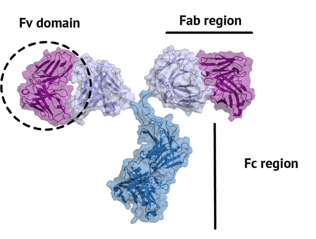
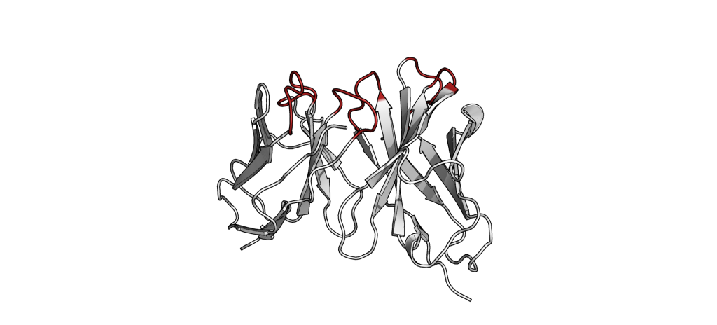
The small part of the Fab region that binds the antigen is called paratope. The part of the antigen that binds to an antibody is called epitope. The paratope consists of six highly flexible loops, known as complementarity-determining regions (CDRs) or hypervariable loops whose sequence and conformation are altered to bind to different antigens. CDRs are shown in red in the figure below:
In this tutorial we will be working with Interleukin-1β (IL-1β) (PDB code 4I1B)) as an antigen and its highly specific monoclonal antibody gevokizumab (PDB code 4G6K) (PDB code of the complex 4G6M).
References:
- R.V. Honorato, M.E. Trellet, B. Jiménez-García, J.J. Schaarschmidt, M. Giulini, V. Reys, P.I. Koukos, J.P.G.L.M. Rodrigues, E. Karaca, G.C.P. van Zundert, J. Roel-Touris, C.W. van Noort, Z. Jandová, A.S.J. Melquiond and A.M.J.J. Bonvin The HADDOCK2.4 web server: A leap forward in integrative modelling of biomolecular complexes. Nature Protoc, 19, 3219–3241 DOI: 10.1038/s41596-024-01011-0 (2024)
ProABC-2 is described here:
- F. Ambrosetti, T.H. Olsed, P.P. Olimpieri, B. Jiménez-García, E. Milanetti, P. Marcatilli and A.M.J.J. Bonvin. proABC-2: PRediction Of AntiBody Contacts v2 and its application to information-driven docking. Bioinformatics, 36, 5107–5108 (2020).
PDB-tools are described here:
- J.P.G.L.M. Rodrigues, J.M.C. Teixeira, M.E. Trellet and A.M.J.J. Bonvin. pdb-tools: a swiss army knife for molecular structures. F1000Research, 7:1961 2018
The local version of PDB-tools can also be found here.
Throughout the tutorial, coloured text will be used to refer to questions or instructions, and/or PyMOL commands.
This is a question prompt: try answering it! This an instruction prompt: follow it! This is a PyMOL prompt: write this in the PyMOL command line prompt!
Setup
In order to run this tutorial you will need to have the following software installed: PyMOL.
Also, if not provided with special workshop credentials to use the HADDOCK portal, make sure to register in order to be able to submit jobs. Use for this the following registration page: https://wenmr.science.uu.nl/auth/register/haddock.
HADDOCK general concepts
HADDOCK (see https://www.bonvinlab.org/software/haddock2.4) is a collection of python scripts derived from ARIA (https://aria.pasteur.fr) that harness the power of CNS (Crystallography and NMR System – https://cns-online.org) for structure calculation of molecular complexes. What distinguishes HADDOCK from other docking software is its ability, inherited from CNS, to incorporate experimental data as restraints and use these to guide the docking process alongside traditional energetics and shape complementarity. Moreover, the intimate coupling with CNS endows HADDOCK with the ability to actually produce models of sufficient quality to be archived in the Protein Data Bank.
A central aspect to HADDOCK is the definition of Ambiguous Interaction Restraints or AIRs. These allow the translation of raw data such as NMR chemical shift perturbation or mutagenesis experiments into distance restraints that are incorporated in the energy function used in the calculations. AIRs are defined through a list of residues that fall under two categories: active and passive. Generally, active residues are those of central importance for the interaction, such as residues whose knockouts abolish the interaction or those where the chemical shift perturbation is higher. Throughout the simulation, these active residues are restrained to be part of the interface, if possible, otherwise incurring in a scoring penalty. Passive residues are those that contribute for the interaction, but are deemed of less importance. If such a residue does not belong in the interface there is no scoring penalty. Hence, a careful selection of which residues are active and which are passive is critical for the success of the docking. The docking protocol of HADDOCK was designed so that the molecules experience varying degrees of flexibility and different chemical environments, and it can be divided in three different stages, each with a defined goal and characteristics:
1. Randomization of orientations and rigid-body minimization (it0)
In this initial stage, the interacting partners are treated as rigid bodies, meaning that all geometrical parameters such as bonds lengths, bond angles, and dihedral angles are frozen. The partners are separated in space and rotated randomly about their centres of mass. This is followed by a rigid body energy minimization step, where the partners are allowed to rotate and translate to optimize the interaction. The role of AIRs in this stage is of particular importance. Since they are included in the energy function being minimized, the resulting complexes will be biased towards them. For example, defining a very strict set of AIRs leads to a very narrow sampling of the conformational space, meaning that the generated poses will be very similar. Conversely, very sparse restraints (e.g. the entire surface of a partner) will result in very different solutions, displaying greater variability in the region of binding.
See animation of rigid-body minimization (it0):
2. Semi-flexible simulated annealing in torsion angle space (it1)
The second stage of the docking protocol introduces flexibility to the interacting partners through a three-step molecular dynamics-based refinement in order to optimize interface packing. It is worth noting that flexibility in torsion angle space means that bond lengths and angles are still frozen. The interacting partners are first kept rigid and only their orientations are optimized. Flexibility is then introduced in the interface, which is automatically defined based on an analysis of intermolecular contacts within a 5Å cut-off. This allows different binding poses coming from it0 to have different flexible regions defined. Residues belonging to this interface region are then allowed to move their side-chains in a second refinement step. Finally, both backbone and side-chains of the flexible interface are granted freedom. The AIRs again play an important role at this stage since they might drive conformational changes.
See animation of semi-flexible simulated annealing (it1):
3. Refinement in Cartesian space with explicit solvent (water)
Note: This stage was part of the standard HADDOCK protocol up to (and including) v2.2. As of v2.4 it is no longer performed by default but the user still has the option of enabling it. In its place, a short energy minimisation is performed instead. The final stage of the docking protocol immerses the complex in a solvent shell so as to improve the energetics of the interaction. HADDOCK currently supports water (TIP3P model) and DMSO environments. The latter can be used as a membrane mimic. In this short explicit solvent refinement the models are subjected to a short molecular dynamics simulation at 300K, with position restraints on the non-interface heavy atoms. These restraints are later relaxed to allow all side chains to be optimized.
See animation of refinement in explicit solvent (water):
The performance of this protocol of course depends on the number of models generated at each step. Few models are less probable to capture the correct binding pose, while an exaggerated number will become computationally unreasonable. The standard HADDOCK protocol generates 1000 models in the rigid body minimization stage, and then refines the best 200 – regarding the energy function - in both it1 and water. Note, however, that while 1000 models are generated by default in it0, they are the result of five minimization trials and for each of these the 180º symmetrical solution is also sampled. Effectively, the 1000 models written to disk are thus the results of the sampling of 10.000 docking solutions.
The final models are automatically clustered based on a specific similarity measure - either the positional interface ligand RMSD (iL-RMSD) that captures conformational changes about the interface by fitting on the interface of the receptor (the first molecule) and calculating the RMSDs on the interface of the smaller partner, or the fraction of common contacts (FCC) (current default) that measures the similarity of the intermolecular contacts. For RMSD clustering, the interface used in the calculation is automatically defined based on an analysis of all contacts made in all models.
Extracting antibody amino acid sequence to gain information about the paratope
Nowadays there are several computational tools that can identify the paratope from the provided antibody sequence. In this tutorial we will use the one developed in our group ProABC-2. ProABC-2 uses a convolutional neural network to identify not only residues which are located in the paratope region but also the nature of interactions they are most likely involved in (hydrophobic or hydrophilic). The work is described in Ambrosetti, et al Bioinformatics, 2020.
Using PDB tools to extract the amino acid sequence
In this step we will make use of the PDB-tools webserver. PDB-tools webserver is a powerful tool that enables you to edit pdbs quickly and painlessly without any scripting knowledge. It does not require registration and individual commands can be joined together into a pipeline which can be saved for future use.
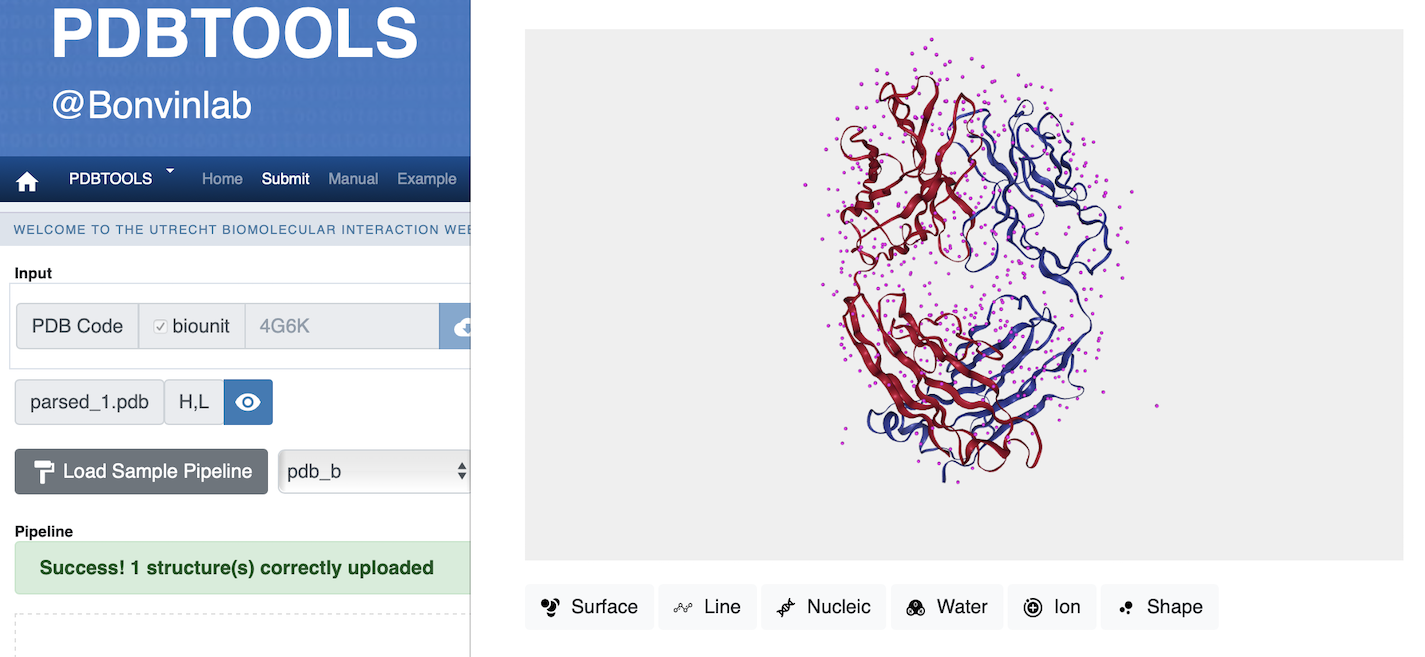
First open your web browser to go to https://wenmr.science.uu.nl/pdbtools/ and choose Submit a pipeline.
Here, we fetch the antibody structure directly by typing 4G6K in the PDB Code field.
Check the field for biounit, to download the functional form of the molecule.
After the structure is fetched properly, we can see that it contains two chains: H (heavy chain) and L (light chain). When we click on the eye icon we visualise the full Fab part of gevokizumab, with heavy chain in red and light chain in blue. Waters are shown as pink spheres and can be shown/hidden by selectin the Water button.
Now we will split our antibody into two (ligh and heavy) chains, to prepare the input for ProABC-2.
Choose ‘pdb_splitchain’ from the Pre-processing panel and click on +Add a new block.
Then we need to clean our pdb structure by removing all water, ion or other non-protein atoms as a result from the crystallisation process.
Choose ‘pdb_delhetatm’ and click on +Add a new block.
Finally we convert this structural PDB file into a fasta sequence file.
Choose ‘pdb_tofasta’ and click on +Add a new block
One can find the explanation of the commands by hovering over them with the mouse.
Once you have all commands in our pipeline click on Run this.
On the result page we can see two output files, each corresponding to one chain of the protein. For each the command used to run PBD-tools is also given.
Save output_1_0.fasta as heavy_chain.fasta and output_1_1.fasta as light_chain.fasta.
If you wish to save the pipeline after this step, click on Download JSON pipeline.
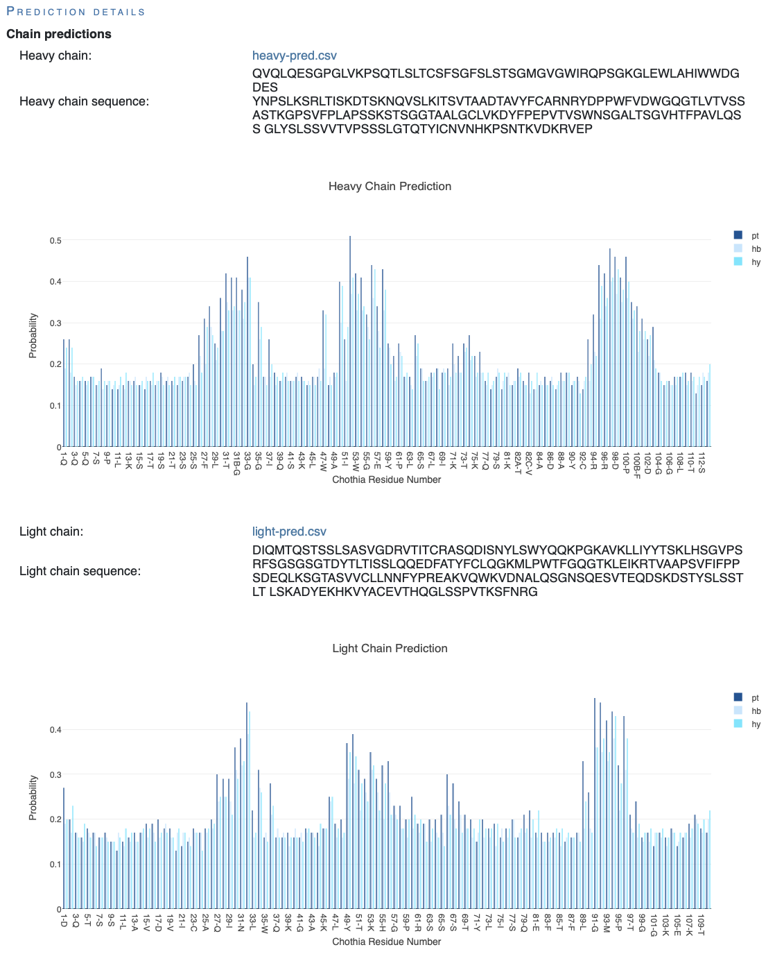
Using ProABC-2 to identify the paratope
Because of security issues we had to discontinue the ProABC-2 service. The code is however freely available from our GitHub repository, which also include a docker container to run the server. The ProABC-2 prediction will be provided below, so no need to run the predictions at this stage.
Note: ProABC-2 uses the Chothia numbering scheme for antibodies and only shows results for the antibody Fv domains. Insertions created by this numbering scheme (e.g. 82A,82B,82C) cannot be processed by HADDOCK directly and renumbering is necessary before starting the docking. Extracting active residues corresponding to this renumbered structures can be done locally as described in Ambrosetti, et al ArXiv, 2020. For simplicity we have already done this for you in this tutorial.
See the result page of ProABC-2 with 4G6K:
Inspecting and preparing the antibody for docking
Using PDB tools to renumber the antibody and to extract the variable domain (Fv)
In this step we again use the PDB-Tools web server to fetch the PDB file, repeating the first two steps shown above to extract the variable region of the antibody.
Check the field for biounit, to download the functional form of the molecule.
Tip: After fetching/uploading a pdb one can use a very useful command pdb_wc. If we run only this command upon splitting the chains (pdb_splitchain), we get all essential information about the number of chains, residues or atoms in your pdb. Here is the result of running pdb_splitchain and pdb_wc for 4G6K.
Output for parsed_1_H.pdb
No. models:	1
No. chains:	1	(   1.0/model)
No. residues:	220	( 220.0/model)
No. atoms:	1649	(1649.0/model)
No. HETATM:	262
Multiple Occ.:	False
Res. Inserts:	False
Output for parsed_1_L.pdb
No. models:	1
No. chains:	1	(   1.0/model)
No. residues:	212	( 212.0/model)
No. atoms:	1642	(1642.0/model)
No. HETATM:	248
Multiple Occ.:	False
Res. Inserts:	False
For docking, we should remove all non-relevant atoms, e.g. crystallised waters and other small molecules that might originate from the crystalliation buffer. This can be done in PBD-Tools with:
Choose ‘pdb_delhetatm’ and click on +Add a new block.
pdb_chain will rename all chains to a given value. This step is especially important with the local version of HADDOCK, where each binding partner has to consist of one chain. The HADDOCK2.4 webserver does this step automatically for you.
Choose ‘pdb_chain’ and click on +Add a new block. Type A into the starting field
Until now each chain of the pdb starts with residue number 1. This can be confusing and cannot be processed by HADDOCK. In next step we renumber the antibody so that each residue has its unique number.
Choose ‘pdb_reres’ and click on +Add a new block Type 1 into the starting field
Now we extract the variable domain of the antibody. From the results of ProABC-2 we see that the variable domains of both light and heavy chain represent roughly the first 110-120 residues of each chain. Since we know that the first-heavy chain contains 220 residues, the second chain starts with 221.
Choose ‘pdb_selres’ and click on +Add a new block Type 1:120,221:327 into the selection field
Since we truncated the antibody, the numbering is no longer sequential. Let’s add another renumbering step to fix this!
Choose ‘pdb_reres’ and click on +Add a new block Type 1 into the starting field
Checking this box “cleans up” the pdb and removes any irrelevant lines that could disturb following residue renumbering.
Note that one can download or upload an existing pipeline which can be used repeatedly.
Once you have all commands in our pipeline click on Run this.
The final command should look like:
$ cat parsed_1.pdb | pdb_delhetatm.py | pdb_chain.py -A | pdb_reres.py -1 | pdb_selres.py -1:120,221:327 | pdb_reres.py -1 | pdb_tidy.py
One can also download the complete pipeline here.
Save output_1.pdb as 4G6K_fv.pdb . If you wish to save the pipeline after this step, click on Download JSON pipeline.
Using HADDOCK to model the antibody-antigen complex
Registration / Login
If not provided with special workshop credentials, in order to start the submission you need first to register. For this go to https://wenmr.science.uu.nl/haddock2.4/ and click on Register.
To start the submission process, you are prompted for our login credentials. After successful validation of the credentials you can proceed to the structure upload under Submit a new job.
Note: The blue bars on the server can be folded/unfolded by clicking on the arrow on the left
Scenario 1: No information about the epitope is available
In previous steps we have identified the paratope residues of the antibody. Those can now be used to guide the docking. The second part of the puzzle is the information about the antigen interface, which is often not available. In this this scenario, we assume nothing is known about the epitope. Therefore, we will treat the entire surface of the antigen as potential interface. Since we have to sample the entire surface of the antigen, we need to increase the sampling.
Submission and validation of structures
For this we will make use of the HADDOCK 2.4 interface of the HADDOCK web server.
In this stage of the submission process we can upload the antibody structure we previously prepared with PDB-tools and the IL-1β structure.
-
Step 1: Define a name for your docking run in the field “Job name”, e.g. 4G6M-Ab-Ag-surface.
-
Step 2: Select the number of molecules to dock, in this case the default 2.
-
Step 3: Input the first protein PDB file. For this unfold the Molecule 1 - input if not already unfolded.
First molecule: where is the structure provided? -> “I am submitting it” Which chain to be used? -> All (for this particular case) PDB structure to submit -> Browse and select 4G6K_fv.pdb (the result file of the second PDB-tools pipeline)
Note: Leave all other options to their default values.
- Step 4: Input the second protein PDB file. For this, unfold the Molecule 2 - input if not already unfolded. The structure of Interleukin-1β (IL-1β) is already prepared and can be downloaded here.
First molecule: where is the structure provided? -> “I am submitting it” Which chain to be used? -> All (for this particular case) PDB structure to submit -> Browse and select 4I1B-matched.pdb (the file you saved)
- Step 5: Click on the Next button at the bottom left of the interface. This will upload the structures to the HADDOCK webserver where they will be processed and validated (checked for formatting errors). The server makes use of Molprobity to check side-chain conformations, eventually swap them (e.g. for asparagines) and define the protonation state of histidine residues.
Definition of restraints
If everything went well, the interface window should have updated itself and it should now show the list of residues for molecules 1 and 2. We will be making use of the text boxes below the residue sequence of every molecule to specify the list of active residues to be used for the docking run.
- Step 6: Specify the active residues for the first molecule. For this, unfold the “Molecule 1 - parameters” if not already unfolded. Here fill in the residues of CDR loops that we extracted beforehand for you following the local version of the protocol. Note that the numbers are similar (not identical) to the results of ProABC-2.
Active residues (directly involved in the interaction) -> 26,27,28,29,30,31,32,55,56,57,101,102,103,106,108,146,147,148,150,151,152,170,172,212,213,214,215 Automatically define passive residues around the active residues -> uncheck (checked by default)
Note that in this list of active residues from the HV loops we have filtered out the residues that are not or poorly solvent accessible. We used for this the relative solvent accessibility as calculated by NACCESS freely available to non-profit users, or its open-source software alternative FreeSASA.
- Step 7: Specify the active residues for the second molecule. For this, unfold the “Molecule 2 - parameters” if not already unfolded.
Automatically define passive residues around the active residues -> uncheck (checked by default) Automatically define surface residues as passive -> check
In the entry “If you specified that surface residues will be defined automatically as passive, selection will use the following RSA (relative solvent accessibility) cutoff” leave 0.40 as cutoff. Leave the other options to their default parameters.
Increasing sampling
-
Step 8: Click on the Next button on the bottom of the page.
-
Step 9: Because we have not defined concrete epitope but selected the entire surface of the antigen instead, we need to increase the sampling. For this, unfold the Sampling parameters menu:
Number of structures for rigid body docking -> 10000 Number of structures for semi-flexible refinement -> 400 Number of structures for the final refinement -> 400
- Step 10: Increase the number of models to analyse to 400. For this open the Analysis parameter menu:
Number of structures to analyze -> 400
Job submission
This interface allows us to modify many parameters that control the behaviour of HADDOCK, but in our case, the default values are all appropriate. It also allows us to download the input structures of the docking run (in the form of a tgz archive) and a haddockparameter file which contains all the settings and input structures for our run (in json format). We strongly recommend downloading this file as it will allow you to repeat the run by uploading it into the file upload inteface of the HADDOCK webserver. The haddockparameter file also serves as a run input reference. It can be edited to change a few parameters and repeat the run without going through the whole menu process again.
- Step 11: Click on the Submit button at the bottom left of the interface.
Upon submission you will be presented with a web page which also contains a link to the previously mentioned haddockparameter file as well as some information about the status of the run.
Scenario 2: A loose definition of the epitope is known
In this scenario, additionally to the CDR residues of the antibody, a loose definition of the epitope residues of the antigen will be used to guide the docking. Here, we define the epitope on the antigen as all residues within 9Å from the antibody in the complex reference structure (pdb code 4G6M), filtered by their relative solvent accessibility (≥0.40) upon the removal of the antibody. This is of course an artificial scenario. In a real case the epitope might have been identified for example from NMR titration experiments (see Bonus below), H/D exchange experiments, …
Submission and validation of structures
We again make us of the HADDOCK 2.4 interface of the HADDOCK web server.
In this stage of the submission process we can upload the structures we previously prepared with PyMOL.
-
Step 1: Define a name for your docking run in the field “Job name”, e.g. 4G6M-Ab-Ag.
-
Step 2: Select the number of molecules to dock, in this case the default 2.
-
Step 3: Input the first protein PDB file. For this, unfold the Molecule 1 - input if not already unfolded.
First molecule: where is the structure provided? -> “I am submitting it” Which chain to be used? -> All (for this particular case) PDB structure to submit -> Browse and select 4G6K_fv.pdb (the result file of the second PDB-tools pipeline)
Note: Leave all other options to their default values.
- Step 4: Input the second protein PDB file. For this, unfold the Molecule 2 - input if not already unfolded. The structure of Interleukin-1β (IL-1β) is already prepared and can be downloaded here.
First molecule: where is the structure provided? -> “I am submitting it” Which chain to be used? -> All (for this particular case) PDB structure to submit -> Browse and select 4I1B-matched.pdb (the file you saved)
- Step 5: Click on the Next button at the bottom left of the interface. This will upload the structures to the HADDOCK webserver where they will be processed and validated (checked for formatting errors). The server makes use of Molprobity to check side-chain conformations, eventually swap them (e.g. for asparagines) and define the protonation state of histidine residues.
Definition of restraints
If everything went well, the interface window should have updated itself and it should now show the list of residues for molecules 1 and 2. We will be making use of the text boxes below the residue sequence of every molecule to specify the list of active residues to be used for the docking run.
- Step 6: Specify the active residues for the first molecule. For this, unfold the “Molecule 1 - parameters” if not already unfolded.
Active residues (directly involved in the interaction) -> 26,27,28,29,30,31,32,55,56,57,101,102,103,106,108,146,147,148,150,151,152,170,172,212,213,214,215 Automatically define passive residues around the active residues -> uncheck (checked by default)
Note that in this list of active residues from the HV loops we have filtered out the residues that are not or poorly solvent accessible. We used for this the relative solvent accessibility as calculated by NACCESS freely available to non-profit users, or its open-source software alternative FreeSASA.
Note: The web interface allows you to visualize the selected active residues.
- Step 7: Specify the residues for the second molecule. For this, unfold the “Molecule 2 - parameters” if not already unfolded.
Since we have a rather loose definition of the interface, we will input the corresponding residues in this case as passive, which means they will not be penalized if not making contacts.
Automatically define passive residues around the active residues -> uncheck (checked by default) Passive residues (surrounding surface residues) -> 22,46,47,48,64,71,72,73,74,75,82,84,85,86,87,91,92,95,114,116,117
- Step 8: Click on the Next button on the bottom of the page. Since we have defined interface on both interaction partners, we can keep the default sampling parameters.
Job submission
This interface allows us to modify many parameters that control the behaviour of HADDOCK, but in our case, the default values are all appropriate. It also allows us to download the input structures of the docking run (in the form of a tgz archive) and a haddockparameter file which contains all the settings and input structures for our run (in json format). We strongly recommend downloading this file as it will allow you to repeat the run by uploading it into the file upload inteface of the HADDOCK webserver. The haddockparameter file also serves as a run input reference. It can be edited to change a few parameters and repeat the run without going through the whole menu process again. An excerpt of this file is shown here:
- Step 9: Click on the Submit button at the bottom left of the interface.
Upon submission, you will be presented with a web page which also contains a link to the previously mentioned haddockparameter file as well as some information about the status of the run.
Analysing the results
Once your run has completed you will be presented with a result page showing the cluster statistics and some graphical representation of the data (and if registered, you will also be notified by email). If using course credentials provided to you, the number of models generated will have been decreased (250/50/50) to allow the runs to complete within a reasonable amount of time.
In case you don’t want to wait for your runs to be finished, precalculated runs can be found here:
- Scenario 1: 4G6M-Ab-Ag-surface
- Scenario 2: 4G6M-Ab-Ag
How many clusters are generated?
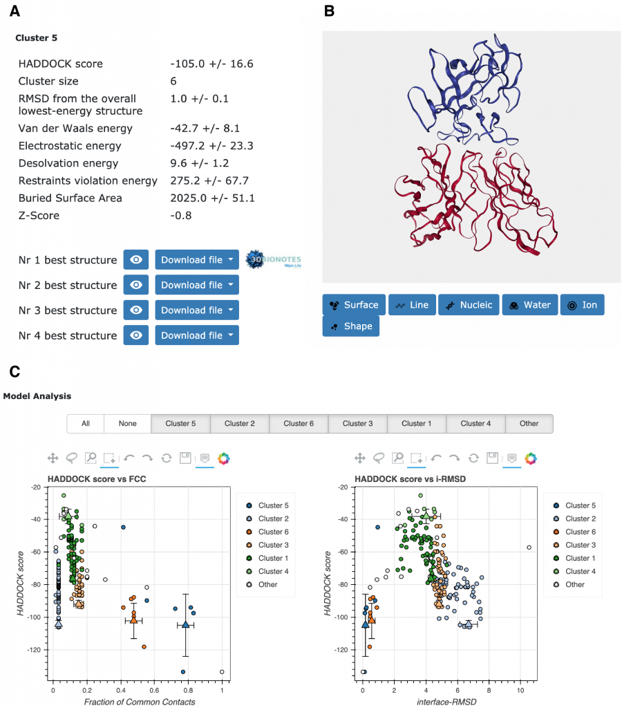
In the figure below you can see different parts of the result page.
In A the result page reports the number of clusters and for the top 10 clusters also the related statistics (HADDOCK score, Size, RMSD, Energies, BSA and Z-score). While the name of the clusters is defined by their size (cluster 1 is the largest, followed by cluster 2 etc..) the top 10 clusters are selected and sorted according to the average HADDOCK score of the best 4 models of each cluster, from the lowest (best) HADDOCK score to the highest (worst).
In B the visualization option of the various models is shown. You can visualize online a model by clicking on the eye icon, or download those for further analysis.
In C a view of some graphical representation of the results shown at the bottom of the page under Model analysis is shown. Distribution of various measures (HADDOCK score, van der Waals energy, …) as a function of the Fraction of Common Contact with- and RMSD from the best generated model (the best scoring model) are shown. The models are color-coded by the cluster they belong to. You can turn on and off specific clusters, but also zoom in on specific areas of the plot.
The bottom graphs in Cluster analysis show you the distribution of components of the HADDOCK score (Evdw, Eelec and Edesol) for the various clusters.
The ranking of the clusters is based on the average score of the top 4 members of each cluster. The score is calculated as:
HADDOCKscore = 1.0 * Evdw + 0.2 * Eelec + 1.0 * Edesol + 0.1 * Eair
where Evdw is the intermolecular van der Waals energy, Eelec the intermolecular electrostatic energy, Edesol represents an empirical desolvation energy term adapted from Fernandez-Recio et al. J. Mol. Biol. 2004, and Eair the AIR energy.
Consider the cluster scores and their standard deviations. Is the top ranked cluster significantly better than the second one? (This is also reflected in the z-score).
In case the scores of various clusters are within standard deviation from each other, all should be considered as a valid solution for the docking. Ideally, some additional independent experimental information should be available to decide on the best solution. In this case we do have such a piece of information: crystal structure of the complex.
Note: The type of calculations performed by HADDOCK does have some chaotic nature, meaning that you will only get exactly the same results unless you are running on the same hardware, operating system and using the same executable. The HADDOCK server makes use of EGI/EOSC high throughput computing (HTC) resources to distribute the jobs over a wide grid of computers worldwide. As such, your results might look slightly different from what is presented in the example output pages. That run was run on our local cluster. Small differences in scores are to be expected, but the overall picture should be consistent.
Visualisation
In the CAPRI (Critical Prediction of Interactions) Méndez et al. 2003 experiment, one of the parameters used is the Ligand root-mean-square deviation (l-RMSD) which is calculated by superimposing the structures onto the backbone atoms of the receptor (the antibody in this case) and calculating the RMSD on the backbone residues of the ligand (the antigen). To calculate the l-RMSD it is possible to either use the software Profit or Pymol. For the sake of convenience we provide you with a renumbered reference structure 4G6M-matched.pdb, which can be downloaded here.
Scenario 1: No information about the epitope is available
In case you do not want to wait for the run to be finished, you can have a look at the completed run here.
Download and save to disk the first model of each cluster (use the PDB format)
Note that you can download all cluster models at once by clicking on download all cluster files just above the first cluster statistics.
Then start PyMOL and load each cluster representative:
File menu -> Open -> select cluster4_1.pdb
Repeat this for each cluster and 4G6M-matched.pdb. Once all files have been loaded, type in the PyMOL command window:
show cartoon
util.cbc
hide lines
Let’s then superimpose all models on chain A (receptor) of the first reference structure and calculate RMSD of chain B (ligand):
Repeat the align and rms commands for each cluster representative.
In CAPRI, the L-RMSD value defines the quality of a model:
- incorrect model: L-RMSD>10Å
- acceptable model: L-RMSD<10Å
- medium quality model: L-RMSD<5Å
- high quality model: L-RMSD<1Å
What is the quality of these models? Did any model pass the acceptable threshold?
Note: You can turn on and off a cluster by clicking on its name in the right panel of the PyMOL window.
Let’s now check if the active and passive residues which we defined are actually part of the interface. In the PyMOL command window type:
Since have defined the entire surface of the antigen as passive, the actual epitope is not compelled to be at the interface. It can still happen, however this pose won’t be preferred to any other.
Scenario 2: A loose definition of the epitope is known
In case you do not want to wait for the run to be finished, you can have a look at the completed run here.
Now we can compare our docking without any information about the epitope with a run where the epitope was defined.
Inspect the result page. How is the HADDOCK score different from the previous run?
Proceed the same way as in Scenario 1. Download the best models of individual clusters and compare them to 4G6M-matched.
Since interacting residues were defined in both binding partners, the docking positions these residues at the interface. fulfilling these restraints.
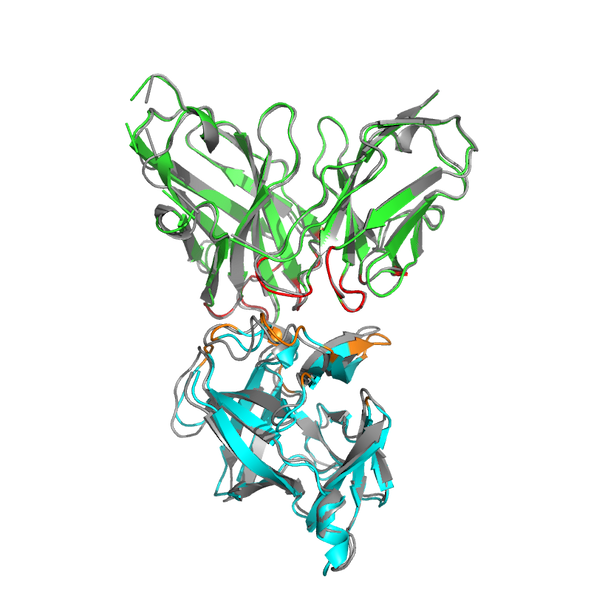
Here you can see an overlay of model 1 of the best cluster (in our case cluster 4) with the crystal structure of the complex (4G6M-matched.pdb).
See the L-RMSDs for clusters in both scenarios:
* 4G6M-Ab-Ag cluster4_1  HADDOCKscore [a.u.] = -112.8 +/- 4.5 ligand-RMSD =  1.86Å
* 4G6M-Ab-Ag cluster5_1  HADDOCKscore [a.u.] = -105.0 +/- 3.8 ligand-RMSD =  9.23Å
* 4G6M-Ab-Ag cluster3_1  HADDOCKscore [a.u.] = -101.0 +/- 2.8 ligand-RMSD = 24.23Å
* 4G6M-Ab-Ag cluster1_1  HADDOCKscore [a.u.] =  -85.9 +/- 2.0 ligand-RMSD = 12.15Å
* 4G6M-Ab-Ag cluster2_1  HADDOCKscore [a.u.] =  -73.4 +/- 1.5 ligand-RMSD = 17.01Å

* 4G6M-Ab-Ag-surface cluster6_1   HADDOCKscore [a.u.] = -101.1 +/-  4.3 ligand-RMSD = 22.92Å
* 4G6M-Ab-Ag-surface cluster8_1   HADDOCKscore [a.u.] =  -99.0 +/-  1.9 ligand-RMSD = 18.78Å
* 4G6M-Ab-Ag-surface cluster7_1   HADDOCKscore [a.u.] =  -97.6 +/-  1.7 ligand-RMSD = 26.59Å
* 4G6M-Ab-Ag-surface cluster13_1  HADDOCKscore [a.u.] =  -86.2 +/-  4.0 ligand-RMSD = 27.59Å
* 4G6M-Ab-Ag-surface cluster2_1   HADDOCKscore [a.u.] =  -84.8 +/-  2.4 ligand-RMSD = 25.01Å
* 4G6M-Ab-Ag-surface cluster5_1   HADDOCKscore [a.u.] =  -84.7 +/-  4.7 ligand-RMSD = 21.39Å
* 4G6M-Ab-Ag-surface cluster22_1  HADDOCKscore [a.u.] =  -84.4 +/-  6.7 ligand-RMSD = 23.90Å
* 4G6M-Ab-Ag-surface cluster15_1  HADDOCKscore [a.u.] =  -72.0 +/-  8.8 ligand-RMSD = 23.60Å
* 4G6M-Ab-Ag-surface cluster10_1  HADDOCKscore [a.u.] =  -71.3 +/-  2.7 ligand-RMSD = 24.33Å
* 4G6M-Ab-Ag-surface cluster21_1  HADDOCKscore [a.u.] =  -70.4 +/-  7.5 ligand-RMSD = 25.10Å
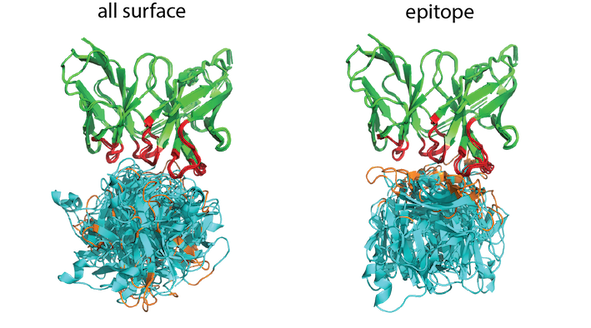
See the overlaid clusters for different scenarios:
Bonus - using NMR titration data to guide the docking
The article describing the crystal structure of the antibody-antigen complex we modelled also reports on experimental NMR chemical shift titration experiments to map the binding site of the antibody on Interleukin-1β. The residues affected by binding are listed in Table 5 of Blech et al. JMB 2013:
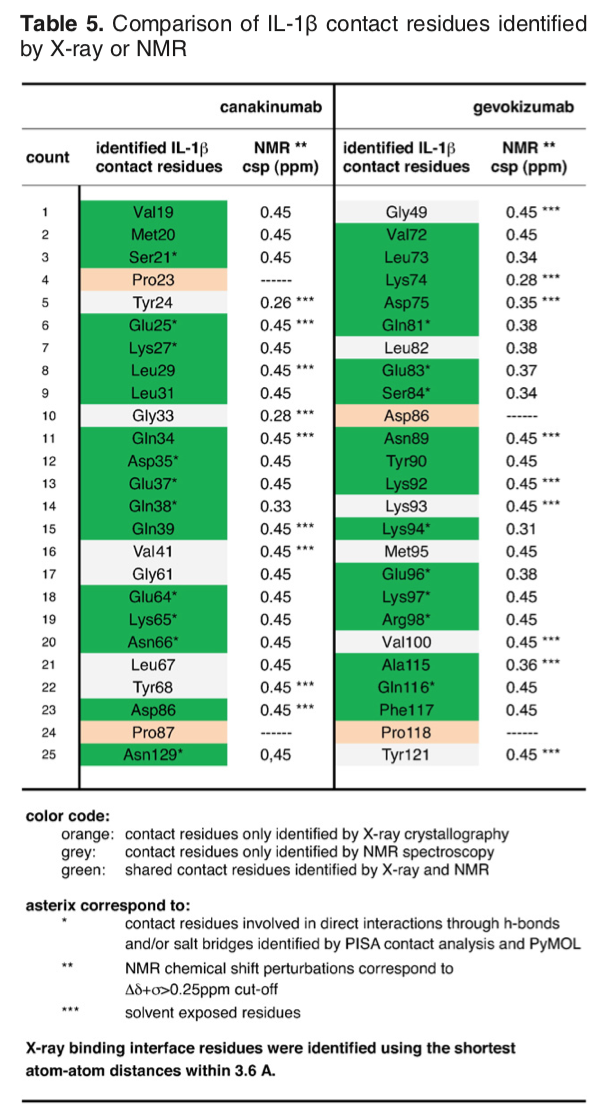
These residues could be used as active residues for Interleukin-1β, leaving HADDOCK define automatically the passive residues around them. Note that the structure we are using for the docking has a numbering shifted by -2. The list of active residues to give to HADDOCK would thus become:
70,71,72,73,81,82,87,88,90,92,94,95,96,113,114,115
The results of such a docking run can be found here.
How do the scores compare with those of scenario 2 above?
Does the top cluster have a score significantly lower than the second best?
Does it contain near native models (l-RMSD <10Å)? (Use PyMol for this analysis)
See the L-RMSDs for the NMR-based clusters:
* 4G6M-Ab-Ag-NMR cluster3_1  HADDOCKscore [a.u.] = -130.2 +/-  3.6 ligand-RMSD =  2.73Å
* 4G6M-Ab-Ag-NMR cluster5_1  HADDOCKscore [a.u.] = -119.8 +/- 14.7 ligand-RMSD =  7.61Å
* 4G6M-Ab-Ag-NMR cluster2_1  HADDOCKscore [a.u.] = -109.4 +/-  2.5 ligand-RMSD = 24.26Å
* 4G6M-Ab-Ag-NMR cluster1_1  HADDOCKscore [a.u.] =  -90.8 +/-  1.4 ligand-RMSD = 11.71Å
* 4G6M-Ab-Ag-NMR cluster4_1  HADDOCKscore [a.u.] =  -75.5 +/-  4.4 ligand-RMSD = 17.70Å
* 4G6M-Ab-Ag-NMR cluster6_1  HADDOCKscore [a.u.] =  -73.4 +/-  7.1 ligand-RMSD = 22.74Å
Conclusions
We have demonstrated the antibody-antigen docking guided with and without the knowledge about epitope. Always check and compare multiple clusters, don’t blindly trust the cluster with the best HADDOCK score! This tutorial is a nice example that the more reliable information is used, the better the results of docking will be.
Congratulations!
You have completed this tutorial. If you have any questions or suggestions, feel free to contact us via email or asking a question through our support center.
And check also our education web page where you will find more tutorials!