

LightDock+HADDOCK membrane proteins tutorial
This tutorial consists of the following sections:
- Introduction
- LightDock general concepts
- Setup/Requirements
- Data preparation
- LightDock simulation
- HADDOCK Refinement
- Analysis
- Conclusions
- Congratulations!
Introduction
This tutorial demonstrates the use of LightDock for predicting the structure of membrane receptor–soluble protein complex using the topological information provided by the membrane to guide the modeling process. The resulting LightDock models are then refined using HADDOCK2.4 webserver. We will be following the protocol described in Roel-Touris et al, 2020.
Membrane proteins are among the most challenging systems to study with experimental structural biology techniques, thus computational techniques such as docking might offer invaluable insights on the modeling of those systems.
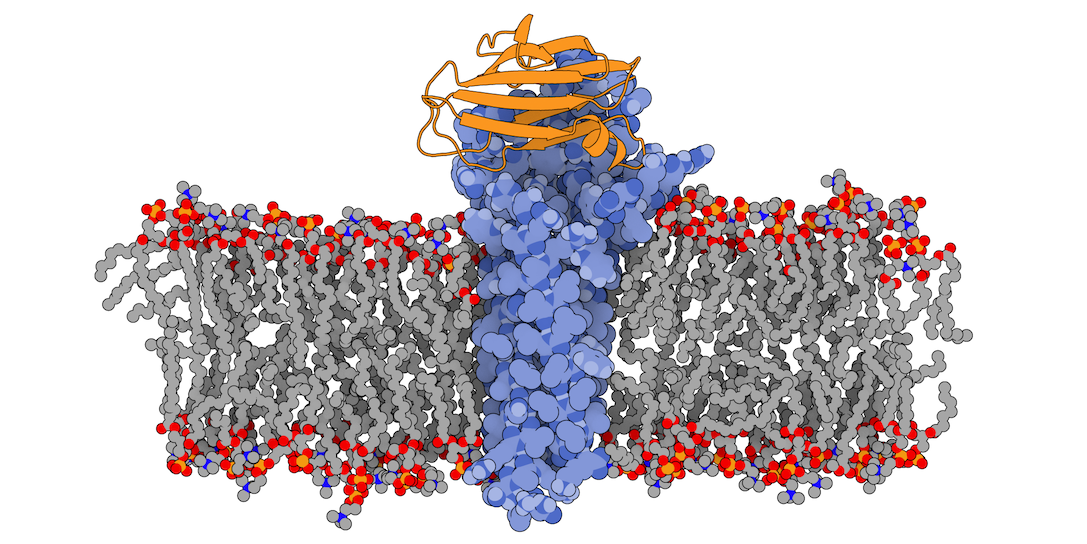
In this tutorial we will be working with the crystal structure of Mus musculus Claudin-19 transmembrane protein (PDB code 3X29, chain A) in complex with the unbound C-terminal fragment of the Clostridium perfringens Enteroxin (PDB code 2QUO, chain A). The PDB code of the complex is 3X29 (chains A and B).
3X29 complex is one of the cases covered in the MemCplxDB membrane protein complex benchmark (Koukos et al, 2018). Despite not being one of the most challenging cases covered in the benchmark in terms of flexibility, its relatively small size will help us describing the complete modeling protocol in the short time intended for a tutorial.
For this tutorial we will make use of the HADDOCK2.4 webserver and LightDock software.
- R.V. Honorato, M.E. Trellet, B. Jiménez-García, J.J. Schaarschmidt, M. Giulini, V. Reys, P.I. Koukos, J.P.G.L.M. Rodrigues, E. Karaca, G.C.P. van Zundert, J. Roel-Touris, C.W. van Noort, Z. Jandová, A.S.J. Melquiond and A.M.J.J. Bonvin The HADDOCK2.4 web server: A leap forward in integrative modelling of biomolecular complexes. Nature Protoc, 19, 3219–3241 DOI: 10.1038/s41596-024-01011-0 (2024)
The integrative approach followed in this tutorial is described here:
- J. Roel-Touris, B. Jimenez-Garcia and A.M.J.J. Bonvin. Integrative modeling of membrane-associated protein assemblies. Nat. Commun., 11, 6210 (2020).
LightDock docking framework is described in the following publications:
-
J. Roel-Touris, A.M.J.J. Bonvin and B. Jimenez-Garcia. LightDock goes information-driven. Bioinformatics, 36:3 950-952 (2020).
-
B. Jimenez-Garcia, J. Roel-Touris, M. Romero-Durana, M. Vidal, D. Jimenez-Gonzalez, J. Fernandez-Recio. LightDock: a new multi-scale approach to protein-protein docking. Bioinformatics, 34:1 49-55 (2018).
Throughout the tutorial, colored text will be used to refer to questions or instructions, commands to be executed in the terminal, and/or PyMOL commands.
This is a question prompt: try answering it! This an instruction prompt: follow it! This is a PyMOL prompt: write this in the PyMOL command line prompt! This is a Linux prompt: insert the commands in the terminal!
LightDock general concepts
LightDock is a macromolecular docking software written in the Python programming language, designed as a framework for rapid prototyping and test of scientific hypothesis in structural biology. It was designed to be easily extensible by users and scalable for high-throughput computing (HTC). LightDock is capable of modeling backbone flexibility of molecules using anisotropic model networks (ANM) and the energetic minimization is based on the Glowworm Swarm Optimization (GSO) algorithm.
LightDock protocol is divided in two main steps: setup and simulation. On setup step, input PDB structures for receptor and ligand partners are parsed and prepared for the simulation. Moreover, a set of swarms is arranged around the receptor surface. Each of these swarms represents an independent simulation in LightDock where a fixed number of agents, called glowworms, encodes for a possible receptor-ligand pose. During the simulation step, each of these glowworms will sample a given region of the energetic landscape depending on its neighboring glowworms.
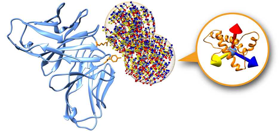
Swarms on the receptor surface can be easily filtered according to regions of interest. Figure 2 shows an example where only two swarms have been calculated to focus on two residues of interest on the receptor partner (depicted in orange). On this tutorial we will explore this capability in order to filter out incompatible transmembrane binding regions in membrane complex docking.
For more information about LightDock, please visit the tutorials section.
Setup/Requirements
In order to run this tutorial you will need to have the following software installed: LightDock, pdb-tools and PyMOL.
Also, if not provided with special workshop credentials to use the HADDOCK portal, make sure to register in order to be able to submit jobs. Use for this the following registration page: https://haddock.science.uu.nl/auth/register/haddock.
Installing LightDock
LightDock is distributed as a Python package through the Python Package Index (PyPI) repository.
Command line
Installing LightDock is as simple as creating a virtual environment for Python 3.6+ and running pip command (make sure your instances of virtualenv and pip are for Python 3.6+ versions). We will install the version 0.9.2post1 of LightDock which is the first released version with support for the membrane protocol and execution in Jupyter Notebooks (see next section):
virtualenv venv
source venv/bin/activate
pip install numpy && pip install lightdock==0.9.2post1
If the installation finished without errors, you should be able to execute LightDock in the terminal:
and to see an output similar to this:
lightdock3 0.9.2post1
Jupyter Notebook and Google Colab
Another option to use LightDock is through Google Colaboratory (“Colab” for short) which allows you to write and execute Python in the browser using notebooks. In case of choosing this option, simply execute in a new notebook in the first cell the following command:
!pip install lightdock==0.9.2post1
Installing PDB-Tools
PDB-Tools is a set of Python scripts for manipulating PDB files following the philosophy of one script, one task. For different manipulating tasks on a PDB file, the procedure would be to pipe the different PDB-Tools scripts to accomplish the different tasks.
PDB-Tools is distributed as a PyPI package. To install it, simply:
or alternatively in a Google Colab notebook:
Tutorial Notebook
We have prepared a Colab Notebook ready to be imported. Download it: tutorial.ipynb
In case of using the provided Colab notebook, go to the Colab site and upload the provided notebook (see A):
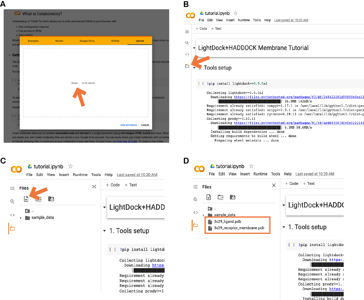
Once imported, click on the icon pointed in (B) and upload the required files as marked in (C) by the orange arrow. The two required files (3x29_receptor_membrane.pdb and 3x29_ligand.pdb) should appear now as in (D).
Then, run one by one each of the code cells as several libraries will be installed in the first code cells.
Data preparation
We will make use of the 3X29 complex simulated in a membrane lipid bilayer from the MemProtMD database (Newport et al., 2018).
First, browse the 3X29 complex page at MemProtMD and locate the Data Download section.
Download the PDB file corresponding to the Coarse-grained snapshot (MARTINI representation)
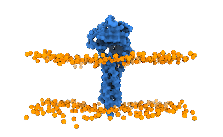
This file in PDB format contains the MARTINI coarse-grained (CG) representation of the phospholipid bilayer membrane and the protein complex. We will use the phosphate beads as the boundary for the transmembrane region for filtering the sampling region of interest in LightDock.
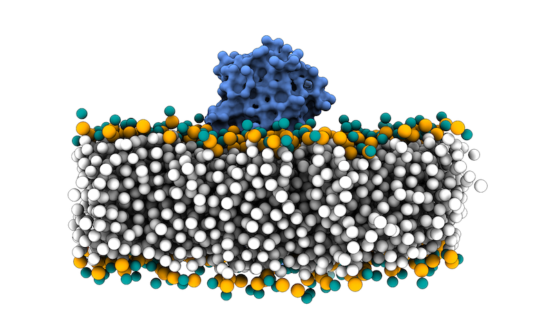
We have prepared a Python script to parse, rename and remove non-necessary beads for the membrane protocol in LightDock: prepare4lightdock.py. You will need to execute it in your terminal using the 3x29_default_dppc-coarsegrained.pdb PDB file as input:
python3 prepare4lightdock.py 3x29_default_dppc-coarsegrained.pdb membrane_cg.pdb
The output of this script is the membrane_cg.pdb PDB file (Figure 4).
The last step will be to open the just generated membrane_cg.pdb file in PyMOL to align the atomistic representation of the 3X29 receptor partner to the membrane CG bilayer:
pymol 3x29_receptor.pdb membrane_cg.pdb
Now execute the following commands on PyMOL to align the membrane with the atomistic receptor and saving the resulting PDB structure:
align 3x29_receptor and name CA, membrane_cg and name CA remove membrane_cg and name CA save 3x29_receptor_membrane.pdb, all
The last PyMOL command will save the aligned atomistic 3X29 receptor to the CG lipid bilayer: 3x29_receptor_membrane.pdb.
LightDock simulation
Simulation set up
The fist step in any LightDock simulation is setup. We will make use of lightdock3_setup.py command to initialize our 3X29 membrane simulation and the required input data is:
Use the lightdock3_setup.py command to set up the LightDock simulation:
lightdock3_setup.py 3x29_receptor_membrane.pdb 3x29_ligand.pdb --noxt --noh --membrane
In short, we are indicating to the setup command to use 3x29_receptor_membrane.pdb as the receptor partner, 3x29_ligand.pdb as the ligand, to skip NOXT and hydrogen atoms and to detect membrane beads with the --membrane flag. The output of the command should look similar to this:
[lightdock3_setup] INFO: Ignoring OXT atoms
[lightdock3_setup] INFO: Ignoring Hydrogen atoms
[lightdock3_setup] INFO: Reading structure from 3x29_receptor_membrane.pdb PDB file...
[pdb] WARNING: Possible problem: [SideChainError] Incomplete sidechain for residue GLN.61
[pdb] WARNING: Possible problem: [SideChainError] Incomplete sidechain for residue GLN.63
[pdb] WARNING: Possible problem: [SideChainError] Incomplete sidechain for residue LYS.65
[pdb] WARNING: Possible problem: [SideChainError] Incomplete sidechain for residue LEU.66
[pdb] WARNING: Possible problem: [SideChainError] Incomplete sidechain for residue ASP.68
[pdb] WARNING: Possible problem: [SideChainError] Incomplete sidechain for residue HIS.76
[pdb] WARNING: Possible problem: [SideChainError] Incomplete sidechain for residue MET.95
[pdb] WARNING: Possible problem: [SideChainError] Incomplete sidechain for residue MET.102
[pdb] WARNING: Possible problem: [SideChainError] Incomplete sidechain for residue LYS.103
[pdb] WARNING: Possible problem: [SideChainError] Incomplete sidechain for residue LYS.115
[pdb] WARNING: Possible problem: [SideChainError] Incomplete sidechain for residue ARG.117
[lightdock3_setup] INFO: 1608 atoms, 601 residues read.
[lightdock3_setup] INFO: Ignoring OXT atoms
[lightdock3_setup] INFO: Ignoring Hydrogen atoms
[lightdock3_setup] INFO: Reading structure from 3x29_ligand.pdb PDB file...
[lightdock3_setup] INFO: 933 atoms, 117 residues read.
[lightdock3_setup] INFO: Calculating reference points for receptor 3x29_receptor_membrane.pdb...
[lightdock3_setup] INFO: Reference points for receptor found, skipping
[lightdock3_setup] INFO: Done.
[lightdock3_setup] INFO: Calculating reference points for ligand 3x29_ligand.pdb...
[lightdock3_setup] INFO: Reference points for ligand found, skipping
[lightdock3_setup] INFO: Done.
[lightdock3_setup] INFO: Saving processed structure to PDB file...
[lightdock3_setup] INFO: Done.
[lightdock3_setup] INFO: Saving processed structure to PDB file...
[lightdock3_setup] INFO: Done.
[lightdock3_setup] INFO: Calculating starting positions...
[lightdock3_setup] INFO: Generated 62 positions files
[lightdock3_setup] INFO: Done.
[lightdock3_setup] INFO: Number of calculated swarms is 62
[lightdock3_setup] INFO: Preparing environment
[lightdock3_setup] INFO: Done.
[lightdock3_setup] INFO: LightDock setup OK
In previous versions of LightDock, the number of swarms of the simulated was given by the user (typically around 400), but since version 0.9.0, the number of swarms of the simulation is automatically calculated depending on the surface area of the receptor structure. However, the number of swarms can be fixed by the user using the -s flag for reproducibility of old results purpose. Another difference with previous versions is that the number of glowworms is now default to 200. This value has been extensively tested on our previous work, but it may be defined by the user as well using the -g flag.
A complete list of lightdock3_setup.py command options might be obtained executing the command without arguments or with the --help flag:
usage: lightdock3_setup [-h] [-s SWARMS] [-g GLOWWORMS] [--seed_points STARTING_POINTS_SEED] [--noxt] [--noh] [--verbose_parser] [-anm] [--seed_anm ANM_SEED] [-ar ANM_REC]
                        [-al ANM_LIG] [-r restraints] [-membrane] [-transmembrane] [-sp] [-sd SURFACE_DENSITY] [-sr SWARM_RADIUS]
                        receptor_pdb_file ligand_pdb_file
lightdock3_setup: error: the following arguments are required: receptor_pdb_file, ligand_pdb_file
The setup command has generated several files and directories:
What is the content of the setup.json file?
What does the init directory contains?
We may visualize the distribution of swarms over the receptor:
pymol lightdock_3x29_receptor_membrane.pdb init/swarm_centers.pdb
Is this a regid-body or a flexible simulation?
Running the simulation
The simulation is ready to run at this point. The number of swarms after focusing on the cytosolic region of the membrane is of 62.
LightDock optimization strategy (using the GSO algorithm) is agnostic of the scoring function (force-field). There are several scoring functions available at LightDock, from atomistic to coarse-grained. In this tutorial we will make use of fastdfire, which is the implementation of DFIRE using the Python C API and the default if no scoring function is specified by the user. Find here a complete list of the current supported scoring functions by LightDock.
Simulation is the most time-consuming part of the protocol. For that reason, we will only simulate one of the 62 total swarms. Pick a swarm number between [0..61] and use that id in the -l argument:
lightdock3.py setup.json 100 -c 1 -s fastdfire -l 60
In the command above, we specify the JSON file of the simulation (setup.json), the number of steps of the simulation (100), the number of CPU cores to use (-c 1), the scoring function (-s fastdfire). If no -l argument is provided, the protocol would simulate all the swarms.
For your convenience, you can download the full run as a compressed file (45MB).
Once the simulation has finished, navigate to the swarm_60 directory (or the one you have selected) and list the directory.
How many gso_* files have been generated? Which one corresponds to the last step of the simulation?
Generating models
Once the simulation has finished successfully, it is time to generate the predicted models. For each swarm, there is a gso_100.out file containing the information to generate as many models as glowworms were defined in the simulation (200 in this tutorial). The command in charge of generating the models is lgd_generate_conformations.py.
Pick a swarm folder and generate the 200 models simulated as in step 100:
lgd_generate_conformations.py 3x29_receptor_membrane.pdb 3x29_ligand.pdb swarm_60/gso_100.out 200
You should see an output similar to this:
[generate_conformations] INFO: Reading ../lightdock_3x29_receptor_membrane.pdb receptor PDB file...
[pdb] WARNING: Possible problem: [SideChainError] Incomplete sidechain for residue GLN.61
[pdb] WARNING: Possible problem: [SideChainError] Incomplete sidechain for residue GLN.63
[pdb] WARNING: Possible problem: [SideChainError] Incomplete sidechain for residue LYS.65
[pdb] WARNING: Possible problem: [SideChainError] Incomplete sidechain for residue LEU.66
[pdb] WARNING: Possible problem: [SideChainError] Incomplete sidechain for residue ASP.68
[pdb] WARNING: Possible problem: [SideChainError] Incomplete sidechain for residue HIS.76
[pdb] WARNING: Possible problem: [SideChainError] Incomplete sidechain for residue MET.95
[pdb] WARNING: Possible problem: [SideChainError] Incomplete sidechain for residue MET.102
[pdb] WARNING: Possible problem: [SideChainError] Incomplete sidechain for residue LYS.103
[pdb] WARNING: Possible problem: [SideChainError] Incomplete sidechain for residue LYS.115
[pdb] WARNING: Possible problem: [SideChainError] Incomplete sidechain for residue ARG.117
[generate_conformations] INFO: 1608 atoms, 601 residues read.
[generate_conformations] INFO: Reading ../lightdock_3x29_ligand.pdb ligand PDB file...
[generate_conformations] INFO: 933 atoms, 117 residues read.
[generate_conformations] INFO: Read 200 coordinate lines
[generate_conformations] INFO: Generated 200 conformations
Clustering models
To remove very similar and redundant models in the same swarm, we will cluster the 200 generated models:
lgd_cluster_bsas.py swarm_60/gso_100.out
After a verbose output of the command above, a new file cluster.repr is generated inside the swarm_60 folder. This file should look like this:
0:3:26.80832:115:lightdock_115.pdb
1:9:24.45152:42:lightdock_42.pdb
2:62:22.70320:37:lightdock_37.pdb
3:35:20.35832:0:lightdock_0.pdb
4:41:16.69347:38:lightdock_38.pdb
5:3:15.71026:79:lightdock_79.pdb
6:7:13.89057:72:lightdock_72.pdb
7:7:11.84427:164:lightdock_164.pdb
8:1: 8.69611:92:lightdock_92.pdb
9:1: 2.92199:137:lightdock_137.pdb
10:22:-0.00771:95:lightdock_95.pdb
11:2:-24.59441:93:lightdock_93.pdb
12:7:-31.35821:57:lightdock_57.pdb
Each line represents a different cluster and lines are sorted from best to worst energy. For each line, there is information about the cluster id, the number of structures in the cluster, the best energy of the cluster, the glowworm id of the model with best energy and the PDB file name of the structure with best energy.
Open the best predicted model for this swarm in PyMOL and have a look.
pymol swarm_60/lightdock_115.pdb
How does this model look in general? What about the side chains?
HADDOCK Refinement
HADDOCK (see https://www.bonvinlab.org/software/haddock2.4) is a collection of python scripts derived from ARIA that harness the power of CNS (Crystallography and NMR System – https://cns-online.org) for structure calculation of molecular complexes. What distinguishes HADDOCK from other docking software is its ability, inherited from CNS, to incorporate experimental data as restraints and use these to guide the docking process alongside traditional energetics and shape complementarity. Moreover, the intimate coupling with CNS endows HADDOCK with the ability to actually produce models of sufficient quality to be archived in the Protein Data Bank. In this tutorial we will make use of HADDOCK for removing clashes at the interface of protein complexes generated by rigid-body docking approaches.
Data preparation
The first step to refine out top predicted models by LightDock will be to prepare a multi-model ensemble PDB file containing those top predicted models.
-
First, download and decompress the provided complete run.
-
Using
pdb-tools, we will removeMMBfake bead residues, copy the chain ID into the segid field and finally creating an ensemble of the top 20 models (we provide the generated top20_ensemble.pdb for your convenience):
Please note that the structures are located inside the clustered directory.
HADDOCK2.4 web server
We will make use of the HADDOCK2.4 web interface to set up the final refinement step of the membrane protocol. Please make sure you are already registered and authenticated on the HADDOCK2.4 server. To start the submission select the Input data tab at https://wenmr.science.uu.nl/haddock2.4/submit.
Input data
-
Step1: Define a name for your docking run in the field “Job name”, e.g. 3x29-Lightdock-CG-refine.
-
Step2: Select the number of molecules to dock, in this case the default 2.
-
Step3: Input the first protein PDB file. For this unfold the Molecule 1 - input if it isn’t already unfolded.
First molecule: where is the structure provided? -> “I am submitting it” Which chain to be used? -> A (for this particular case) PDB structure to submit -> Browse and select top20_ensemble.pdb (the file you edited to modify the histidine) Do you want to coarse-grain your molecule? -> Switch on
Note: Leave all other options to their default values.
- Step4: Input the second protein PDB file. For this unfold the Molecule 2 - input if it isn’t already unfolded.
First molecule: where is the structure provided? -> “I am submitting it” Which chain to be used? -> B (for this particular case) PDB structure to submit -> Browse and select top20_ensemble.pdb (the file you saved)
- Step 5: Click on the “Next” button at the bottom left of the interface. This will upload the structures to the HADDOCK webserver where they will be processed and validated (checked for formatting errors). The server makes use of Molprobity to check side-chain conformations, eventually swap them (e.g. for asparagines) and define the protonation state of histidine residues.
Input parameters
- Step 6: Click on the “Next” button at the bottom left of the interface. Leave everything as if in this second step form and simply click on Next. This is a step intended for defining residues involved in binding for docking. Ignore as well any warning about the protonation of the system if it is the case.
Docking parameters
In this third and final step, we will need to set several options on three main sections: Distance restraints, Sampling parameters and Advanced sampling parameters.
- Step 7: Modify the Distance restraints settings (for this unfold the menu if it isn’t already unfolded).
Turn off Randomly exclude a fraction of the ambiguous restraints (AIRs) Turn on Define surface contact restraints to enforce contact between the molecules
- Step 8: Modify the Sampling parameters (for this unfold the menu if it isn’t already unfolded).
Number of structures for rigid body docking -> 200 Number of trials for rigid body minimisation -> 10 Number of structures for semi-flexible refinement -> 200 Number of structures for the final refinement -> 200 Number of structures to analyze -> 200
- Step 9: Modify the Advanced sampling parameters (for this unfold the menu if it isn’t already unfolded).
Turn off Perform cross-docking Turn off Randomize starting orientations Turn off Perform initial rigid body minimisation Turn off Allow translation in rigid body minimisation Number of MD steps for rigid body high temperature TAD -> 0 Number of MD steps during first rigid body cooling stage -> 0 Number of MD steps during second cooling stage with flexible side-chains at interface -> 0 Number of MD steps during third cooling stage with fully flexible interface -> 0
Job submission
This interface allows us to modify many parameters that control the behavior of HADDOCK but in our case only the above changes are required and all other parameters can be left to their default values.
The interface also allows us to download the input structures of the docking run (in the form of a tgz archive) and a haddockparameter file which contains all the settings and input structures for our run (in JSON format). We strongly recommend to download this file as it will allow you to repeat the run after uploading into the file upload interface of the HADDOCK webserver. It can serve as input reference for the run. This file can also be edited to change a few parameters for example. An excerpt of this file is shown here:
{
  "runname": "3x29-Lightdock-CG-refine",
  "auto_passive_radius" : 6.5,
  "create_narestraints" : true,
  "delenph": true,
  "ranair" : false,
  "cmrest" : false,
  "kcont" : 1.0,
  "surfrest" : true,
  "ksurf" : 1.0,
  "noecv" : false,
  "ncvpart" : 2.0,
  "structures_0" : 500,
  "ntrials" : 5,
  ...
}
- Step 10: Click on the “Submit” button at the bottom left of the interface.
Upon submission you will be presented with a web page which also contains a link to the previously mentioned haddockparameter file as well as some information about the status of the run.
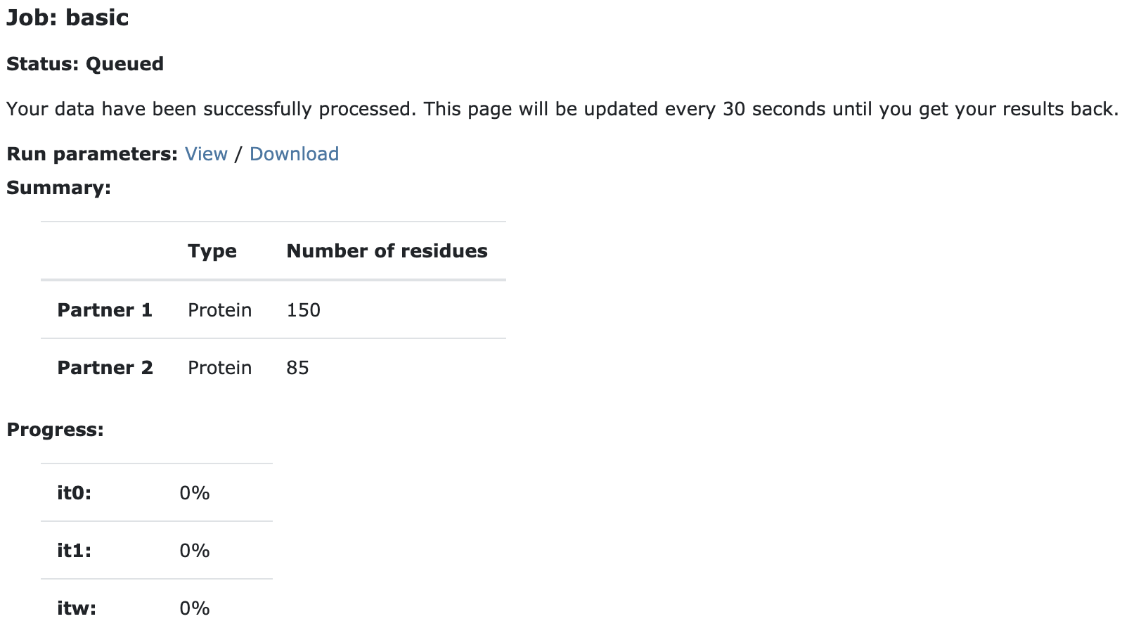
Currently your run should be queued but eventually its status will change to “Running”:
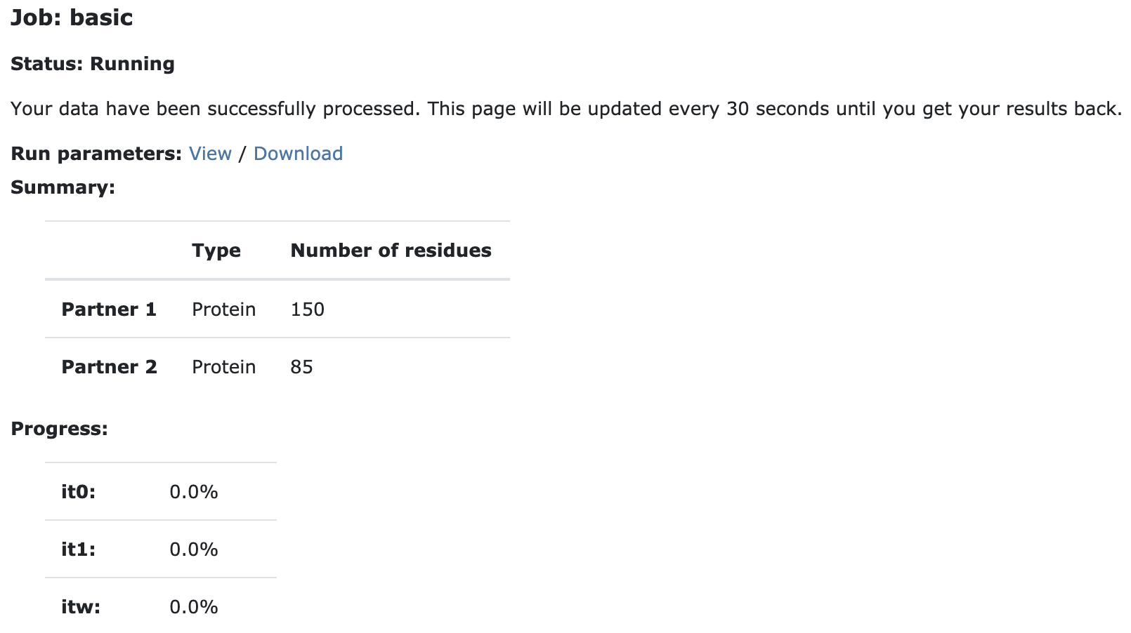
The page will automatically refresh and the results will appear upon completions (which can take between 1/2 hour to several hours depending on the size of your system and the load of the server). You will be notified by email once your job has successfully completed.
Results
Depending on the server load, your refinement job may take some time, but you will receive an email once the job has completed (and the results page will be automatically refreshed).
For your convenience, we provide the refinement job already calculated for you: https://wenmr.science.uu.nl/haddock2.4/run/4242424242/52544-3x29-Lightdock-CG-refine
How many clusters are generated?
Analysis
The results page for the refinement job displays a very useful summary of the energies of the top ranked clusters according to HADDOCK scoring energy. For each cluster, the mean and standard deviation of the HADDOCK score for this cluster is presented. The more the negative this score is, the better. The total energy (and the partial contributions from electrostatics, Van der Waals, desolvation, etc.) will give you a qualitative measure of the goodness of the models, but it is important to notice that the quality of the model does not guarantee it to be a near native solution.
Which metric to your knowledge might classify a model as a near native one?
In the CAPRI (Critical Prediction of Interactions) Méndez et al. 2003 experiment, one of the parameters used is the Ligand root-mean-square deviation (L-RMSD) which is calculated by superimposing the structures onto the backbone atoms of the receptor and calculating the RMSD on the backbone residues of the ligand. To calculate the L-RMSD it is possible to either use the software Profit or Pymol.
We will have a quick look at the top 10 models predicted by LightDock and the top 10 refined by the HADDOCK server and compare them with the 3X29 complex reference. Below you will find a table with the top 10 models according to the LightDock and HADDOCK refinement ranking (click on a name to download):
| Top | Docking (LightDock) | Refinement (HADDOCK) |
|---|---|---|
| 1 | swarm_22_112.pdb | cluster17_1.pdb |
| 2 | swarm_37_11.pdb | cluster2_1.pdb |
| 3 | swarm_39_11.pdb | cluster16_1.pdb |
| 4 | swarm_60_115.pdb | cluster15_1.pdb |
| 5 | swarm_54_167.pdb | cluster14_1.pdb |
| 6 | swarm_37_34.pdb | cluster10_1.pdb |
| 7 | swarm_55_181.pdb | cluster13_1.pdb |
| 8 | swarm_60_42.pdb | cluster11_1.pdb |
| 9 | swarm_37_169.pdb | cluster1_1.pdb |
| 10 | swarm_37_83.pdb | cluster9_1.pdb |
You can also download as compressed files:
Visualizing and aligning in PyMOL
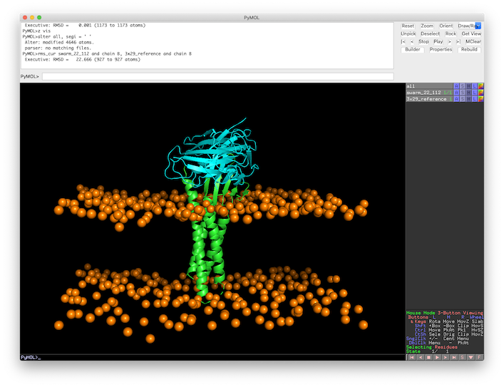
First, open the target and reference structures in PyMOL (in this case top 1 from LightDock ranking):
pymol swarm_22_112.pdb 3x29_reference.pdb
Color by chain (and leave orange the membrane beads): util.cbc color orange, swarm_22_112 and name BJ
Align both structures to the receptor partner (chain A): align swarm_22_112 and chain A, 3x29_reference and chain A
Center visualization: z vis
Calculating L-RMSD in PyMOL
From the alignment of the previous section, we can easily calculate the L-RMSD in PyMOL:
First, remove all segid information to let PyMOL correctly find the target chains:
alter all, segi = ‘ ‘
And now calculate L-RMSD using rms_cur command:
rms_cur swarm_22_112 and chain B, 3x29_reference and chain B
Which leaves a L-RMSD of 22.7Å.
See the calculated L-RMSDs:
HADDOCK:
cluster17_1.pdb  22.531Å
cluster2_1.pdb   13.404Å
cluster16_1.pdb  15.082Å
cluster15_1.pdb  24.945Å
cluster14_1.pdb  24.022Å
cluster10_1.pdb   6.082Å
cluster13_1.pdb  20.806Å
cluster11_1.pdb  15.325Å
cluster1_1.pdb   28.809Å
cluster9_1.pdb   25.826Å

LightDock:
swarm_22_112.pdb 22.551Å
swarm_37_11.pdb  11.850Å
swarm_39_11.pdb  13.424Å
swarm_60_115.pdb  5.735Å
swarm_54_167.pdb 25.031Å
swarm_37_34.pdb  28.587Å
swarm_55_181.pdb 20.470Å
swarm_60_42.pdb  10.801Å
swarm_37_169.pdb 14.894Å
swarm_37_83.pdb  25.857Å
Which is the best structure in terms of L-RMSD in the HADDOCK ranking? And in the LightDock ranking?
In CAPRI, the L-RMSD value defines the quality of a model:
- incorrect model: L-RMSD>10Å
- acceptable model: L-RMSD<10Å
- medium quality model: L-RMSD<5Å
- high quality model: L-RMSD<1Å
What is the quality of these models? Did any model pass the acceptable threshold?
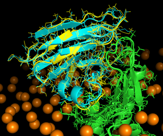
A more in deep look
The best models in terms of quality (L-RMSD) from the LightDock and HADDOCK rankings are swarm_60_115.pdb and cluster10_1.pdb respectively.
Open them in PyMOL, align both structures as explained before and compare both models qualitatively.
How similar do they look to you?
Now use the lines visualization in PyMOL:
Have a close look at the interface of both models. You may visualize atoms clashing in PyMOL:
show sphere, (chain A within 2.5 of chain B) or (chain B within 2.5 of chain A)
What is the best model in terms of clashes?
Conclusions
We have demonstrated the use of membrane information on a protein docking simulation and how to further refine predicted models using a coarse-grained protocol.
It is of paramount importance not to blindly trust docking predictions and rankings. Always inspect the results and predictions and further assess their quality using more metrics and different criteria if possible.
Congratulations!
You have completed this tutorial. If you have any questions or suggestions, feel free to contact us via email or asking a question through our support center.
And check also our education web page where you will find more tutorials!