

PowerFit web server Tutorial
This tutorial consists of the following sections:
- Introduction
- Setup/Requirements
- Inspecting the data
- Rigid body fitting
- Analysing the results
- Final remarks
This tutorial was last updated on 02-03-2026 and is up-to-date
with release v4.0.4.
Introduction
PowerFit is a software developed in our lab to fit atomic resolution structures of biomolecules into cryo-electron microscopy (cryo-EM) density maps. It is open-source and available for download from our Github repository. To facilitate its use, we have developed a web portal for it.
This tutorial demonstrates the use of the PowerFit web server. The server makes use of either local resources on our cluster, using the multi-core version of the software, or GPU-accelerated grid resources of the EGI to speed up the calculations. It only requires a web browser to work and benefits from the latest developments in the software based on a stable and tested workflow. Next to providing an automated workflow around PowerFit, the web server also summarizes and higlights the results in a single page including some visualization of the PowerFit output using MolViewSpec.
The case we will be investigating is a complex between the 30S maturing E. coli ribosome and RsgA, a GTPase. There are models (2YKR) and a cryo-EM density map of around 9.8Å resolution (EMD-1884) available for the complex.
A related tutorial, based on a local installation of PowerFit can be found here. It provides a more detailed analysis of the results of a run with the methyltransferase KsgA, another 30S ribosome partner, and shows how HADDOCK can be used to obtain higher quality models.
The PowerFit and HADDOCK software are described in:
-
G.C.P. van Zundert, M. Trellet, J. Schaarschmidt, Z. Kurkcuoglu, M. David, M. Verlato, A. Rosato and A.M.J.J. Bonvin. The DisVis and PowerFit web servers: Explorative and Integrative Modeling of Biomolecular Complexes.. J. Mol. Biol.. 429(3), 399-407 (2016).
-
G.C.P van Zundert and A.M.J.J. Bonvin. Defining the limits and reliability of rigid-body fitting in cryo-EM maps using multi-scale image pyramids. J. Struct. Biol. 195, 252-258 (2016).
-
G.C.P. van Zundert and A.M.J.J. Bonvin. Fast and sensitive rigid-body fitting into cryo-EM density maps with PowerFit. AIMS Biophysics. 2, 73-87 (2015).
-
G.C.P. van Zundert, A.S.J. Melquiond and A.M.J.J. Bonvin. Integrative modeling of biomolecular complexes: HADDOCKing with Cryo-EM data.. Structure. 23, 949-960 (2015).
Throughout the tutorial, coloured text will be used to refer to questions, instructions, and ChimeraX commands.
This is a question prompt: try answering it! This an instruction prompt: follow it! This is a ChimeraX prompt: write this in the ChimeraX command line prompt!
Setup/Requirements
In order to follow this tutorial you only need a web browser, a text editor, and UCSF ChimeraX
(freely available for most operating systems) on your computer in order to visualise the input and output data.
ChimeraX is a visualization software and popular tool in the cryo-EM community for its volume visualization capabilities.
Further, the required data to run this tutorial should be downloaded here.
Once downloaded, make sure to unpack the archive.
Inspecting the data
Let us first inspect the data we have available, namely the cryo-EM density map and the structures we will attempt to fit.
Using ChimeraX, we can easily visualize and inspect the density and models, mostly through a few mouse clicks.
Open first the density map ribosome-RsgA.map and then the PDB file of the ribosome which is already fitted into the map ribosome.pdb.
ChimeraX will automatically guess their type.
UCSF ChimeraX Menu → File → Open… → Select the file
You can also use the ChimeraX command-line, however you might need to display it first:
UCSF ChimeraX Menu → Tools → Command Line
and type:
open /path/to/ribosome-RsgA.map open /path/to/ribosome.pdb
In the Volume Viewer window, the middle slide bar provides control on the
value at which the isosurface of the density is shown. At high values, the
envelope will shrink while lower values might even display the noise in the map.
We will first make the density transparent, in order to be able to see the fitted structure inside:
Notice that the density becomes transparent providing a better view of the fit
of the ribosome model. On closer inspection, you can also discern a region of
the density that is not accounted for by the ribosome structure alone: This should be the
binding location of RsgA. If you cannot find it you can try to lower the value of the isosurface using the slider in the Volume Viewer window.
Although you could try and manually place the crystal
structure in that region, finding the correct orientation is not
straightforward. PowerFit can help you here as it will exhaustively sample all possible translations and rotations in order to find the best fit, based on an objective score.
Rigid body fitting
PowerFit is a rigid body fitting software that quickly calculates the cross-correlation, a common measure of the goodness-of-fit, between the atomic structure and the density map. It performs a systematic 6-dimensional scan of the three translational and three rotational degrees of freedom. In short, PowerFit will try to systematically fit the structure in different orientations at every position in the map and calculate a cross-correlation score for each of them.
In order to perform the search, PowerFit requires three different things:
a high-resolution atomic structure of the
biomolecule to be fitted (RsgA.pdb), a target cryo-EM density map to fit the
structure in (ribosome-RsgA.map), and the resolution, in Ångstrom, of the
density map (9.8). This is also the minimal required input for the web server in order to setup a run.
To run PowerFit, go to
https://wenmr.science.uu.nl/powerfit
On this page, you will find the most relevant information about the server as well as the links to the local and grid versions of the portal’s submission page.
Step1: Register to the server
Register for getting access to the webserver (or use the credentials provided in case of a workshop).
Registration is not automatic but is usually processed within 12h, so be patient. When you are registered you can use all the software provided in the webserver.
Step2: Define the input files and parameters and submit
Click on the “Submit” menu to access the input form:
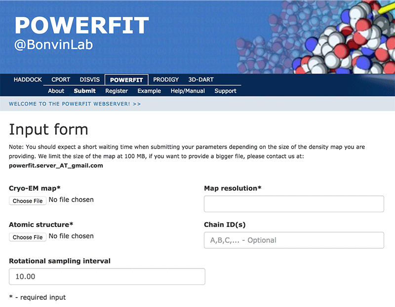
Complete the form by filling the required fields and selecting the respective files (most browsers should also support dragging the files onto the selection button):
Cryo-EM map → ribosome-RsgA.map Map resolution → 9.8 Atomic structure → RsgA.pdb Rotational angle interval → 10.0
Once the fields have been filled in you can submit your job to our server by clicking on “Submit” at the bottom of the page.
If the input fields have been correctly filled you should be redirected to a status page displaying a pop-up message indicating that your run has been successfully submitted. While performing the search, the PowerFit web server will update you on the progress of the job by reloading the status page every 30 seconds. The runtime of this example case is below 5 minutes on our local servers. However the load of the server as well as pre- and post-processing steps might substantially increase the time until the results are available.
While the calculations are running, open a second tab and go to
https://www.bonvinlab.org/powerfit/manual.html
Here, you can have a look at the several features and options of PowerFit and read about the meaning of the various input parameters (including the ones under “Advanced options”).
The rotational sampling interval option is given in degrees and defines how tightly the three rotational degrees of freedom will be sampled. Lower values will cause PowerFit to perform a finer search, at the expense of increased computational time. The default value is 10°, but it can be lowered to 5° for more sensitive searches, or raised to 20° if time is an issue or if there aren’t sufficient computational resources.
Analysing the results
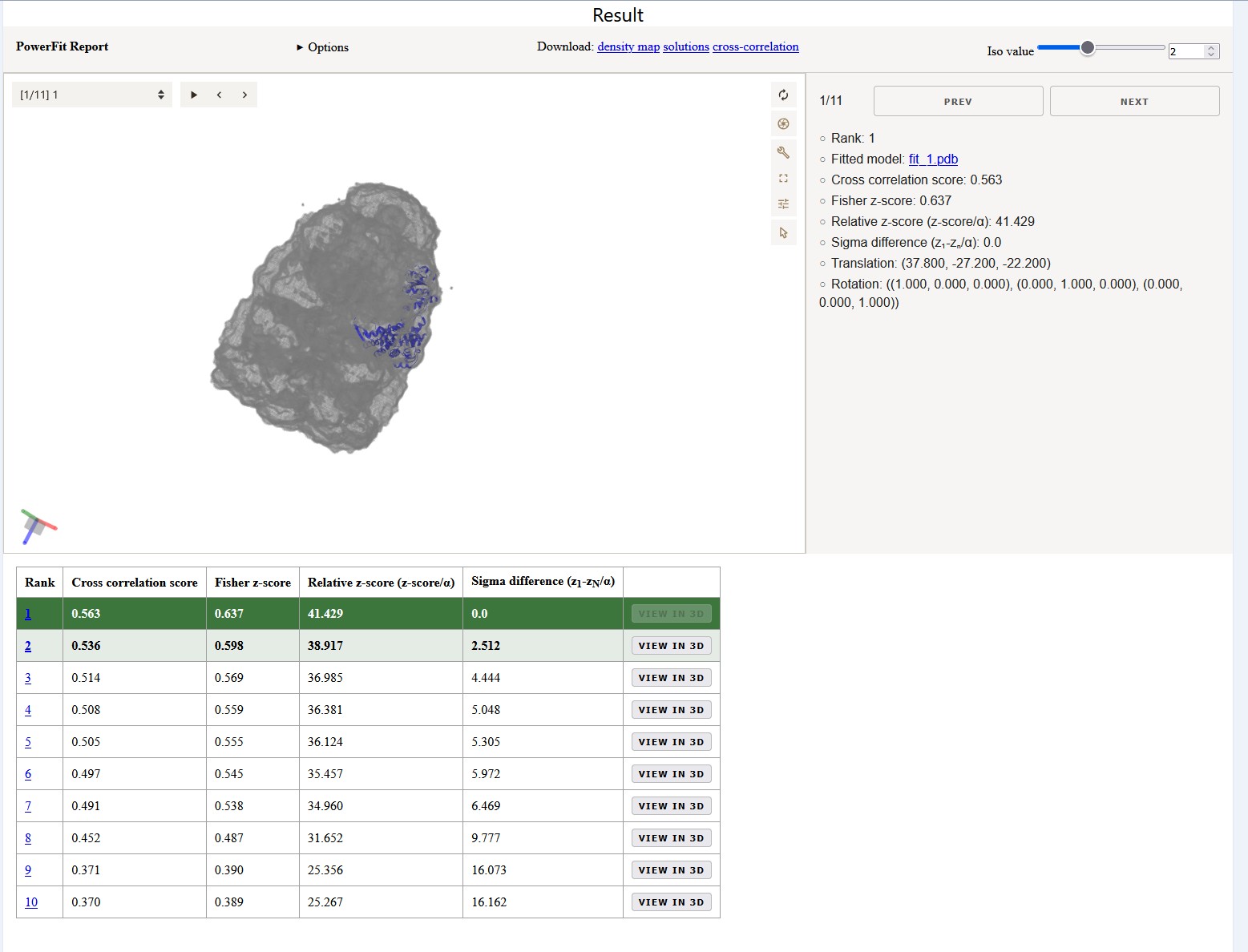
Once your job has completed, and provided you did not close the status page, you will be automatically redirected to the results page (you will also receive an email notification).
On the interactive results page you can look at the top
If you don’t want to wait for your run to complete, you can access the precalculated results of a run submitted with the same input here.
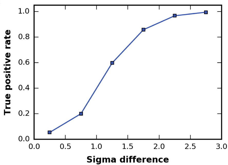
The higher the cross-correlation score the better the fit. But also important is the Fisher z-score (the higher the better),
which, together with its associated number of standard deviations (σ difference), is an excellent indicator of the accuracy of a fit
(see for details van Zundert and Bonvin, J. Struct. Biol. (2016)
and PowerFit help page).
To enhance the interpretation of the results in the Solutions table, the entries are colored in a green gradient up to
a sigma difference of 3.
You can inspect online the results for the top 10 models (different views are provided). However, it is difficult to really appreciate the accuracy of PowerFit and the differences between the solutions with only images. Therefore download the results archive to your computer which is available at the top of your results page.
You will find in it the following files:
fit_N.pdb: the best N fits, judged by the cross-correlation score.solutions.out: all the non-redundant solutions found, ordered by their cross-correlation score. The first column shows the rank, column 2 the correlation score, column 3 and 4 the Fisher z-score and the number of standard deviations; column 5 to 7 are the x, y and z coordinate of the center of the chain; column 8 to 17 are the rotation matrix values.lcc.mrc: a cross-correlation map showing, at each grid position, the highest cross-correlation score found during the search, thus showing the most likely location of the center of mass of the structure.powerfit.log: a log file of the calculation, including the input parameters with date and timing information.
Let us now inspect the solutions in ChimeraX.
Use for this either the Menus or the command line interface as explained before, e.g.:
open /path/to/ribosome-RsgA.map open /path/to/lcc.mrc open /path/to/ribosome.pdb open /path/to/fit_*.pdb
Make the density map transparent again.
The values of the lcc.mrc slider bar correspond to the cross-correlation
score found. In this way, you can selectively visualize regions of high or low
cross-correlation values: i.e., pushing the slider to the right (higher cutoff)
shows only regions of the grid with high cross-correlation scores.
As you can see, PowerFit found quite some local optima, one of which stands out (if the rotational search was tight enough). Further, the 10 best-ranked solutions are centered on regions corresponding to local cross-correlation maxima.
To view each fitted solution individually, open the Model Panel window if it is
not already open
The window shows each model and its associated color that ChimeraX has processed. To show or hide a specific model you can click the box in the column with an eye.
Go through the 10 solutions one by one to asses their goodness-of-fit with the density.
Do you agree with what PowerFit proposes as the best solution?
In a new ChimeraX session, reopen the density map and the fit that you find best.
Use for this either the Menus or the Command Lineoption to load the following files:
ribosome-RsgA.mapribosome.pdbfit_?.pdb
Replace ? by the appropriate solution number.
Note: Make sure to load the files in the specified order for the subsequent commands to work on the correct residues!
You now have combined the ribosome structure with the rigid-body fit of RsgA
calculated by PowerFit, yielding an initial model of the complex. Take a closer look at residues R47 to H51
which are contributing to the interface with the ribosome.
In the command line of ChimeraX, type the following instructions to center your view on these residues and highlight their interactions:
hide #2 atoms
show #2 cartoons
sel #3:47-51
view sel
contacts sel distanceOnly 5.0 makePseudobonds true reveal true
Take some time to inspect the model, paying particular attention to these five
residues and their spatial neighbors.
Are there any clashes between the ribosome and RsgA chains? Show the selection as spheres to visualize this better.
ChimeraX also includes a tool to locally optimize the fit of a rigid structure against a given density map, which can be an additional help on top of the PowerFit calculations. Make the main display window active by clicking on it,
Go to Tools → Volume data → Fit in Map In the newly opened Fit in Map window, select the best-fitted structure of PowerFit (fit_?.pdb) as Fit model and the original density map (ribosome-RsgA.map) as the map. Press Fit to start the optimization.
Does the ChimeraX local fit optimization tool improve the results of PowerFit?
The scoring function used by ChimeraX to estimate the quality of the fit makes
our model worse, increasing the number of clashes between the ribosomal RNA and
RsgA. Click Undo in the Fit in Map window to undo the optimization.
Next, we will try to optimize the fit using the cross-correlation that ChimeraX provides.
Click “Options” and check the “Use map simulated from atoms, resolution” box and fill in 9.8 for resolution. Check the “correlation” radio button and uncheck the “Use only data above contour level from first map”. Press “Fit”.
Does this second strategy improve the quality of the fit? If not, undo it again.
Final remarks
We have demonstrated in this tutorial how to make use of the PowerFit web server to fit atomic structures in cryo-EM map. The obvious limitation of rigid-body fitting is that it cannot account for any conformational changes that the structures might undergo. Further, the low resolution of this particular density map does not allow to identify side-chain atoms. The quality of the fitted models by PowerFit is, therefore, limited. In particular, such models will typically result in a significant clashes at the interface between molecules. Such clashes can be removed by making use of the HADDOCK-EM flexible refinement capabilities. This is demonstrated in the command line version of the PowerFit tutorial and described in:
- G.C.P. van Zundert, A.S.J. Melquiond and A.M.J.J. Bonvin. Integrative modeling of biomolecular complexes: HADDOCKing with Cryo-EM data. Structure. 23, 949-960 (2015).
Thank you for following this tutorial. If you have any questions or suggestions, feel free to contact us via email, or post your question to
our PowerFit forum hosted by the ![]() center of excellence
for computational biomolecular research.
center of excellence
for computational biomolecular research.