

Modelling a covalent inhibitor of cathepsin proteins
This tutorial consists of the following sections:
- Introduction
- Setup
- HADDOCK general concepts
- Scientific context
- Selecting the “best” cathepsin templates for the docking
- Inspecting and preparing Cathepsin K for docking
- Inspecting and preparing the ligand for docking
- Defining the restraints to guide the docking
- Submit your docking run
- Analysis of the docking results
- Visualisation of docked models
- Congratulations!
Introduction
This use-case is a first attempt to blur different software and take on the challenge of “covalent docking”, an important part of pharceutical chemistry that has been barely touched upon by the integrative modelling community. For this tutorial we will make use of the HADDOCK2.2 webserver to predict the three dimensional structures of a covalently bound ligand to cathepsin proteins. A description of our web server can be found in the following publications:
-
G.C.P van Zundert, J.P.G.L.M. Rodrigues, M. Trellet, C. Schmitz, P.L. Kastritis, E. Karaca, A.S.J. Melquiond, M. van Dijk, S.J. de Vries and A.M.J.J. Bonvin. The HADDOCK2.2 webserver: User-friendly integrative modeling of biomolecular complexes. J. Mol. Biol., 428, 720-725 (2015).
-
S.J. de Vries, M. van Dijk and A.M.J.J. Bonvin. The HADDOCK web server for data-driven biomolecular docking. Nature Protocols, 5, 883-897 (2010). Download the final author version here.
Throughout the tutorial, coloured text will be used to refer to questions or instructions and/or PyMOL commands.
This is a question prompt: try answering it! This is an instruction prompt: follow it! This is a PyMol prompt: write this in the PyMol command line prompt! This is a Linux prompt: insert the commands in the terminal!
Setup
In order to run this tutorial you will need to have the following software installed: PyMOL.
Also, if not provided with special workshop credentials to use the HADDOCK portal, make sure to register in order to be able to submit jobs. Use for this our registration page.
If you have questions, feedbacks or recommendations, either during the course of after, please post them on the dedicated topic we created on our interest group forum
HADDOCK general concepts
HADDOCK (see https://www.bonvinlab.org/software/haddock2.4) is a collection of python scripts derived from ARIA (https://aria.pasteur.fr) that harness the power of CNS (Crystallography and NMR System – https://cns-online.org) for structure calculation of molecular complexes. What distinguishes HADDOCK from other docking software is its ability, inherited from CNS, to incorporate experimental data as restraints and use these to guide the docking process alongside traditional energetics and shape complementarity. Moreover, the intimate coupling with CNS endows HADDOCK with the ability to actually produce models of sufficient quality to be archived in the Protein Data Bank.
A central aspect to HADDOCK is the definition of Ambiguous Interaction Restraints or AIRs. These allow the translation of raw data such as NMR chemical shift perturbation or mutagenesis experiments into distance restraints that are incorporated in the energy function used in the calculations. AIRs are defined through a list of residues that fall under two categories: active and passive. Generally, active residues are those of central importance for the interaction, such as residues whose knockouts abolish the interaction or those where the chemical shift perturbation is higher. Throughout the simulation, these active residues are restrained to be part of the interface, if possible, otherwise incurring in a scoring penalty. Passive residues are those that contribute for the interaction, but are deemed of less importance. If such a residue does not belong in the interface there is no scoring penalty. Hence, a careful selection of which residues are active and which are passive is critical for the success of the docking.
The docking protocol of HADDOCK was designed so that the molecules experience varying degrees of flexibility and different chemical environments, and it can be divided in three different stages, each with a defined goal and characteristics:
-
1. Randomization of orientations and rigid-body minimization (it0)
In this initial stage, the interacting partners are treated as rigid bodies, meaning that all geometrical parameters such as bonds lengths, bond angles, and dihedral angles are frozen. The partners are separated in space and rotated randomly about their centres of mass. This is followed by a rigid body energy minimization step, where the partners are allowed to rotate and translate to optimize the interaction. The role of AIRs in this stage is of particular importance. Since they are included in the energy function being minimized, the resulting complexes will be biased towards them. For example, defining a very strict set of AIRs leads to a very narrow sampling of the conformational space, meaning that the generated poses will be very similar. Conversely, very sparse restraints (e.g. the entire surface of a partner) will result in very different solutions, displaying greater variability in the region of binding. -
2. Semi-flexible simulated annealing in torsion angle space (it1)
The second stage of the docking protocol introduces flexibility to the interacting partners through a three-step molecular dynamics-based refinement in order to optimize interface packing. It is worth noting that flexibility in torsion angle space means that bond lengths and angles are still frozen. The interacting partners are first kept rigid and only their orientations are optimized. Flexibility is then introduced in the interface, which is automatically defined based on an analysis of intermolecular contacts within a 5Å cut-off. This allows different binding poses coming from it0 to have different flexible regions defined. Residues belonging to this interface region are then allowed to move their side-chains in a second refinement step. Finally, both backbone and side-chains of the flexible interface are granted freedom. The AIRs again play an important role at this stage since they might drive conformational changes. -
3. Refinement in Cartesian space with explicit solvent (water)
The final stage of the docking protocol immerses the complex in a solvent shell so as to improve the energetics of the interaction. HADDOCK currently supports water (TIP3P model) and DMSO environments. The latter can be used as a membrane mimic. In this short explicit solvent refinement the models are subjected to a short molecular dynamics simulation at 300K, with position restraints on the non-interface heavy atoms. These restraints are later relaxed to allow all side chains to be optimized.
The performance of this protocol of course depends on the number of models generated at each step. Few models are less probable to capture the correct binding pose, while an exaggerated number will become computationally unreasonable. The standard HADDOCK protocol generates 1000 models in the rigid body minimization stage, and then refines the best 200 – regarding the energy function - in both it1 and water. Note, however, that while 1000 models are generated by default in it0, they are the result of five minimization trials and for each of these the 180º symmetrical solution is also sampled. Effectively, the 1000 models written to disk are thus the results of the sampling of 10.000 docking solutions.
The final models are automatically clustered based on a specific similarity measure - either the positional interface ligand RMSD (iL-RMSD) that captures conformational changes about the interface by fitting on the interface of the receptor (the first molecule) and calculating the RMSDs on the interface of the smaller partner, or the fraction of common contacts (current default) that measures the similarity of the intermolecular contacts. For RMSD clustering, the interface used in the calculation is automatically defined based on an analysis of all contacts made in all models.
Scientific context
Osteoporosis affects about 10% of the population in Europe, Japan and North America and its incidence rate is growing with increasing life expectancy. The main feature of osteoporosis is bone loss mediated by osteoclasts and insufficient rebuilding of bone matrix by osteoblasts. A longstanding theory of osteoporosis is that the balance between these two activities has gone off, with bone destruction running ahead. It is very hard to slow down osteoclast activity without slowing down osteoblast activity as well, but one therapy showed promises: the cathepsin K inhibitors.
Cathepsin K is a highly potent cysteine protease expressed in osteoclasts. This enzyme is able to break down collagen, elastin, gelatin and other proteins. It is found almost entirely in this cell type, giving a real hope of targeting osteoclasts selectively. At last, protease inhibitors themselves are a type of small molecule that, in general, give good success in drug discovery. For all those reasons, cathepsin K inhibitors have been studied for more than 20 years and several pharmaceutical companies have currently compounds in clinical trials.
We will use HADDOCK to predict the covalent binding of a small ligand on a protein receptor, using as example a purine nitrile derived inhibitor of cathepsin K (see fig. 1), described in the following publication:
- E. Altmann, S.W. Cowan-Jacob and M. Missbach. Novel Purine Nitrile Derived Inhibitors of the Cysteine Protease Cathepsin K J. Med. Chem (2004)

Figure 1: Purine nitrile derived inhibitor cocrystallized in the cathepsin K active site. PDB code is 1u9v.
One important feature of this inhibitor (PDBeChem code: IHE) is that it can bind three highly homologous cathepsin proteins, with a remarkable affinity:
- Cat K 6 nM IC50
- Cat L 89 nM IC50
- Cat S 150 nM IC50
A lot of three-dimensional structures of cathepsins in the presence of small inhibitors are available in the Protein Data Bank. While the crystal structure of this complex is available from the PDB (1U9V), we will perform our docking from alternate conformations crystallized with alternative ligands.
Selecting the “best” cathepsin templates for the docking
In practice, the structure of the protein can be obtained if:
- Free structures of homologous proteins are known and can be used as templates to model the protein. Typically, sequence similarity, structure resolution and experimental conditions will determine which template is the best to select.
- The unbound structure of the protein is known
- Bound structures of homologous proteins are known and can be used to approximate the bound structure of the receptor.
- Bound structures of the protein with different ligands are known.
Based on our previous experience with the D3R challenges, we decided to use ligand similarity to select a protein template for small molecule docking. The similarity metric that we employ is the widely accepted Tanimoto Coefficient (TC). Given two molecules, A and B, depicted in fig. 2 the TC is defined as follows: \(TC=\frac{C}{A+B-C}\) where TC is the Tanimoto Coefficient, A is the set of atoms of molecule A, B is the set of atoms of molecule B and C is the set of atoms that is shared between the two molecules.

Figure 2: How to calculate TC? Illustration on two ligands used in this tutorial. On the left is the structure of our ligand of interest taken from the reference PDBid 1U9V, and on the right another covalent inhibitor of cathepsin K proteins taken from the PDBid 3KW9
The shared set of atoms is depicted in fig. 3 and it is identified by detecting the Maximum Common Substructure (MCS) of the two molecules.

Figure 3: How to calculate TC? Maximum Common Substructure shared between the two molecules. The shared atoms are highlighted with a blue background.
To illustrate the rich diversity of cathepsins K, L and S structures with inhibitors and their TC differences despite their very high homology, we calculated a pairwise TC matrix (see fig. 4)

Figure 4: Pairwise TC distances between all cathepsins K, L and S structures available in the presence of a small inhibitor
We decided to choose the closest related templates based on their TC.
- CatK -> PDB ID 3KW9 TC=0.25
- CatL -> PDB ID 4AXM TC=0.62
- CatS -> PDB ID 3N4C TC=0.56
In the remaining of this tutorial we will work with Cathepsin K, but you are welcome to repeat all steps with Cathepsin L and S, respectively.
Inspecting and preparing Cathepsin K for docking
We will now inspect the Cathepsin K structure. For this start PyMOL and in the command line window of PyMOL (indicated by PyMOL>) type:
fetch 3KW9
show cartoon
hide lines
show sticks, not chain A
You should see a backbone representation of the protein (corresponding to chain A in the PDB file) with two additional small molecules and crystal waters.
To highlight the binding pocket you can switch to a surface representation of the protein:
sele chain A
show surface, sele
As a preparation step before docking, it is advised to remove any irrelevant water and other small molecules (e.g. small molecules from the crystallisation buffer), however do leave relevant co-factors if present. In this particular example we should delete the two small ligands present in the PDB file and the water molecules. You can remove those in PyMOL by typing:
sele resn HOH
remove sele
sele resn ORG+TFA
remove sele
As final step save the molecule as a new PDB file which we will call: 3KW9-clean.pdb
For this in the PyMOL menu on top select:
File -> Save molecule… Select 3KW9 and click on the save button Name your file 3KW9-clean.pdb and note its location
Inspecting and preparing the ligand for docking
For the ligand, some programs like PRODRG allow you to generate a structure for a chemical directly from a simple sketch in a text editor. However, whenever possible, we advise you to use SMILES or MOL files for the ligand when the atomic coordinates are not available. To illustrate the difficulty of ligand modelling, there is no strict consensus in the algorithms that generate the SMILES strings and each of them choose only one of the main possible strings. For instance, open the PDBeChem page for our cathepsin K inhibitor and look for the SMILES provided (ACDLabs, CACTVS, OpenEye).
Generating and sampling suitable ligand conformations for docking is an art in itself, which we will not cover in this tutorial From our participation to the D3R challenges, we have good experience with the OpenEye Scientific Software suite for which it is possible to request an academic license.
For this tutorial we could download a representive PDB file of our ligand from the PDBeChem database.
This representative conformation is actually the bound form of the ligand from the 1U9V PDB entry we are aiming at reproducing.
This means that effectively in the docking we are going to perform the ligand is in an ideal conformation already.
In order to facilitate later on the analysis of the docking results and the comparison with the reference structure,
we will however extract the ligand coordinates directly from PDB entry 1U9V since in that way the atom names will match.
For this start again PyMol and type:
The last two commands displays the cysteine to which the ligand is covalently bound and zooms on the ligand. Take the time to inspect the structure and look at how the ligand is covalently attached to the protein.
Finally, save the IHE ligand coordinates to file and note its location on disk:
Defining the restraints to guide the docking
Before setting up the docking we need first to generate the distance restraint file for defining the “covalent bond” in a format suitable for HADDOCK. HADDOCK uses CNS as computational engine. A description of the format for the various restraint types supported by HADDOCK can be found in our Nature Protocol paper, Box 4.
Distance restraints are defined as:
assi (selection1) (selection2) distance, lower-bound correction, upper-bound correction
The lower limit for the distance is calculated as: distance minus lower-bound correction and the upper limit as: distance plus upper-bound correction
The syntax for the selections can combine information about chainID - segid keyword -, residue number - resid
keyword -, atom name - name keyword.
Other keywords can be used in various combinations of OR and AND statements. Please refer for that to the online CNS manual.
Here would be an example of an arbitrary distance restraint between the CB carbons of residues 10 and 200 in chains A and B with an allowed distance range between 10 and 20Å:
assi (segid A and resid 10 and name CB) (segid B and resid 200 and name CB) 20.0 10.0 0.0
Let’s now define the distance restraints to represent our covalent bond for docking. We will use for that two distance restraints. The first one will be between the sulfur atom of the targeted cysteine and the reactive nitrile carbon of the ligand with a distance set to 1.8Å ± 0.1Å, consistent with the average length of a simple C-S bond.
The second distance is defined between the CB of the cysteine and the atom adjacent to the reactive nitrile carbon and is meant to impose the proper angular geometry. This distance is set to 2.8Å ± 0.1Å, (as measured in between the CG and CE atoms of a methionine side-chain as reference).
For this we need to create the following distance restraint file:
assign (segid A and name SG and resi 25) (segid B and name C27 and resi 300) 1.8 0.1 0.1
assign (segid A and name CB and resi 25) (segid B and name C27 and resi 300) 2.8 0.1 0.1
The residue number of the ligand is 300. In the file we previously saved, its chain ID is A, but during docking we will define it as molecule B.
You can either create this file yourself using your favorite text editor (BUT NOT Word) or download it from here for convenience.
Submit your docking run
Note that fine-tuning the parameters of the web server to covalently dock a ligand requires the most advanced privilege on the web server. If you did not apply for the “guru” access level yet, it is time to apply for it on our registration portal. If using workshop credentials, you will have “guru” access already.
A problem when trying to “covalently dock” a small ligand is that the van der Waals interactions will typically prevent close proximity of the atoms involved in the covalent bond. To allow the distance restraint to be satisfied, we need to scale down the non-bonded interactions between the specific atoms involved in that covalent bond. For this purpose we created a special Cysteine residue (residue name: CYC), without hydrgogen atom on the sulfur and with significantly reduced VDW parameters for the sulfur atom (scaled down by a factor 10).
You can do it with your favorite text editor, or using the following command in a terminal:
sed s/CYS\ A\ \ 25/CYC\ A\ \ 25/g 3KW9-clean.pdb > 3KW9-clean-CYC.pdb
We will now launch the docking run. For this we will make us of the guru interface of the HADDOCK web server:
https://alcazar.science.uu.nl/services/HADDOCK2.2/haddockserver-guru.html
Note: The blue bars on the server can be folded/unfolded by clicking on the arrow on the right
-
Step1: Define a name for your docking run, e.g. CatK-ligand.
-
Step2: Input the protein PDB file. For this unfold the First Molecule menu.
First molecule: where is the structure provided? -> “I am submitting it” Which chain to be used? -> All (for this particular case) PDB structure to submit -> Choose the clean, modified file you created (3KW9-clean-CYC.pdb)
- Step3: Input the ligand PDB file. For this unfold the Second Molecule menu.
First molecule: where is the structure provided? -> “I am submitting it” Which chain to be used? -> All (for this particular case) PDB structure to submit -> Choose the ligand PDB file you saved (IHE.pdb)
- Step4: Upload the distance restraing file (.tbl). For this unfold the Distance restraints menu.
Upload the tbl file as unambiguous restraints HADDOCK deletes by default all hydrogens except those bonded to a polar atom (N, O). Uncheck this option if you have NOEs or other specific restraints to non-polar hydrogens -> uncheck this option
- Step5: Change the clustering settings. For this unfold the Parameters for clustering menu.
The default clustering method in the HADDOCK2.2 server is fcc-based clustering, which is a measure of similarity of interfaces based on pairwise residue contacts. This method outperforms RMSD-based clustering for large systems, both in term of accuracy and speed. However for ligand docking, interface-RMSD remains the method of choice. Change therefore the clustering method:
Clustering method (RMSD or Fraction of Common Contacts (FCC)) -> RMSD RMSD Cutoff for clustering (Recommended: 7.5A for RMSD, 0.60 for FCC) -> 1Å
- Step 6: Apply some ligand-specific scoring setting. For this unfold the Scoring parameter menu:
Our recommended HADDOCK score settings for small ligands docking are the following:
     HADDOCKscore-it0   = 1.0 Evdw + 1.0 Eelec + 1.0 Edesol + 0.01 Eair - 0.01 BSA

     HADDOCKscore-it1   = 1.0 Evdw + 1.0 Eelec + 1.0 Edesol +  0.1 Eair - 0.01 BSA

     HADDOCKscore-water = 1.0 Evdw + 0.1 Eelec + 1.0 Edesol +  0.1 Eair
This differs from the defaults setting (defined for protein-protein complexes). We recommend to change two weights for protein-ligand docking:
- Step 7: Apply some ligand-specific protocol setting. For this unfold the Advanced sampling parameter menu:
initial temperature for second TAD cooling step with flexible side-chain at the inferface -> 500 initial temperature for third TAD cooling step with fully flexible interface -> 300 number of MD steps for rigid body high temperature TAD -> 0 number of MD steps during first rigid body cooling stage -> 0
- Step 8: You are ready to submit! Enter your username and password (or the course credentials provided to you). Remember that for this interface you do need guru access.
Upon submission you will first be presented with a web page containing a link to the results page, but also an importantly a link to a haddockparameter file (simple text format) containing all settings and input data of your run.
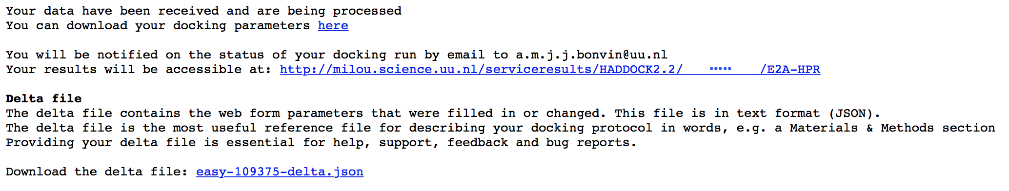
We strongly recommend to save this haddockparameter file since it will allow you to repeat the run by simple upload into the file upload inteface of the HADDOCK webserver. It can serve as input reference for the run. This file can also be edited to change a few parameters for examples. An excerpt of this file is shown here:
HaddockRunParameters (
  runname = 'CatK-IHE',
  auto_passive_radius = 6.5,
  create_narestraints = True,
  delenph = False,
  ranair = False,
  cmrest = False,
  kcont = 1.0,
  surfrest = False,
  ksurf = 1.0,
  noecv = True,
  ncvpart = 2.0,
  structures_0 = 1000,
  ntrials = 5,
...
Click now on the link to the results page. While your input data are being validated and processed the page will show:
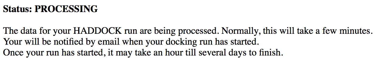
During this stage the PDB and eventually provided restraint files are being validated. Further the server makes use of Molprobity to check side-chain conformations, eventually swap them (e.g. for asparagines) and define the protonation state of histidine residues. Once this has been successfully done, the page will indicated that your job is first QUEUED, and then RUNNING. The page will automatically refresh and the results will appear upon completions (which can take between 1/2 hour to several hours depending on the size of your system and the load of the server). You will be notified by email once your job has successfully completed.
Analysis of the docking results
Once your run has completed you will be presented with a result page showing the cluster statistics and some graphical representation of the data (and if registered, you will also be notified by email). If using course credentials provided to you, the number of models generated will have been decreased to allow the runs to complete within a reasonable amount of time. Because of that, the results might not be very good, although in this particular case, considering we are using distance restraints to model the covalent bond, we would expect that even the limited sampling should generate reasonable models.
We already pre-calculated full docking run for all three cathepsins (meaning that the default number of models has been generated: 1000 for rigid-body docking and 200 for semi-flexible and water refinement). The full runs for the three cathepsins can be accessed at:
- CatK: View here the pre-calculated results
- CatL: View here the pre-calculated results
- CatS: View here the pre-calculated results
Inspect the result pages. How many clusters are generated?
Note: The bottom of the page gives you some graphical representations of the results, showing the distribution of the solutions for various measures (HADDOCK score, van der Waals energy, …) as a function of the RMSD from the best generated model (the best scoring model).
The ranking of the clusters is based on the average score of the top 4 members of each cluster. The score is calculated as:
HADDOCKscore = 1.0 Evdw + 0.1 Eelec + 1.0 Edesol + 0.1 Eair
where Evdw is the intermolecular van der Waals energy, Eelec the intermolecular electrostatic energy, Edesol represents an empirical desolvation energy term adapted from Fernandez-Recio et al. J. Mol. Biol. 2004, and Eair the AIR energy. The cluster numbering reflects the size of the cluster, with cluster 1 being the most populated cluster. The various components of the HADDOCK score are also reported for each cluster on the results web page.
Consider the cluster scores and their standard deviations. Is the top ranked cluster significantly better than the second one? (This is also reflected in the z-score).
In case the scores of various clusters are within standard devatiation from each other, all should be considered as a valid solution for the docking. Ideally, some additional independent experimental information should be available to decide on the best solution.
It is important to emphasize that the HADDOCK score is not consistently in agreement with IC50 values, this is only a mere coincidence and we hope the collaboration with CPMD can greatly improve our predictions to this regard.
Visualisation of docked models
Let’s now visualise the various solutions!
Then start PyMOL and load the cluster representatives:
File menu -> Open -> Select the files …
Repeat this for each cluster. Once all files have been loaded, type in the PyMOL command window:
fetch 1u9v
as cartoon
util.cnc
We now want to highlight the reactive cysteine (position 25) and the covalently bound ligand in sticks. The ligand as residue name IHE. At last, because HADDOCK added hydrogens to all polar and non-polar atoms, we can remove them to facilitate the visual comparison with the reference structure.
show sticks, resn IHE
show stick, resi 25
remove hydrogens
To allow RMSD calculations, we first need to change the chainID of the ligand in the reference structure:
alter (resn IHE and 1u9v), chain="B"
Let’s now superimpose the models on the reference structure 1u9v and calculate the ligand RMSD:
align cluster1_1, 1u9v rms_cur resn IHE and cluster1_1, 1u9v
Repeat this for the various cluster representatives and take note of the ligand RMSD values
See a view of the top models of each cluster for this particular run, superimposed on the reference structure (1U9V in yellow):

Does the best cluster ranked by HADDOCK also correspond to the best (smallest) ligand-RMSD value?
See solution:
 * Cluster1     HADDOCKscore [a.u.] = -68.2 +/- 0.5       ligand-RMSD = 2.04
 * Cluster3     HADDOCKscore [a.u.] = -60.5 +/- 4.3       ligand-RMSD = 2.15
 * Cluster2     HADDOCKscore [a.u.] = -55.3 +/- 1.0       ligand-RMSD = 0.65
Now finally, let’s consider the scores of the three cathepsin-ligand docking runs (CatK, CatL and CatS).
Compare the score of the best cluster with the IC50 values of the ligand
Is there any correlation between docking score and IC50s?
See the IC50 and HADDOCK scores of the three cathepsins:
 * Cat K     IC50 =   6 nM      HADDOCKscore [a.u.] = -68.2 +/- 0.5
 * Cat L     IC50 =  89 nM      HADDOCKscore [a.u.] = -61.2 +/- 1.0
 * Cat S     IC50 = 150 nM      HADDOCKscore [a.u.] = -47.5 +/- 0.1
Note that in general we should not interpret docking scores in terms of binding affinity values. So any correlation observed here does not mean this is generally applicable. In this particular case, considering that the ligand is the same and only rather minor changes are present between the different cathepsin sequences, we do observe a slight correlation. But again, this should not be taken as a rule. We have actually shown that for protein-protein complexes that there is no correlation between the various scoring functions using in docking and binding affinity.
See:
- P.L. Kastritis and A.M.J.J. Bonvin. Molecular origins of binding affinity: Seeking the Archimedean point. Curr. Opin. Struct. Biol., 23, 868-877 (2013).
- P.L. Kastritis and A.M.J.J. Bonvin. On the binding affinity of macromolecular interactions: daring to ask why proteins interact J. R. Soc. Interface, 10, doi: 10.1098/rsif.2012.0835 (2013).
- P. Kastritis and A.M.J.J. Bonvin. Are scoring functions in protein-protein docking ready to predict interactomes? Clues from a novel binding affinity benchmark. J. Proteome Research, 9, 2216-2225 (2010).
Congratulations!
You have completed this tutorial. If you have any questions or suggestions, feel free to post on the dedicated topic on our interest group forum.