

Homology modelling of the mouse MDM2 protein
General Overview
This tutorial is divided into various sections, each representing (roughly) a step of the homology modelling procedure.
- A bite of theory
- Using UniProt to retrieve sequence information
- Finding homologues of known structure using SWISS-MODEL
- Congratulations!
A bite of theory
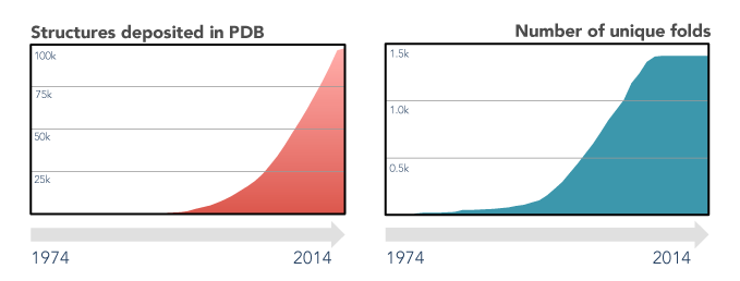
The last decades of scientific advances in the fields of protein biology revealed the extent of both the protein sequence and structure universes. Protein sequences databases currently hold hundreds of millions of entries (source) and are foreseen to continue growing exponentially, driven by high-throughput sequencing efforts. On the other hand, the number of experimental protein structures is three orders of magnitude smaller (source), and that of unique folds has remained virtually unchanged since 2008. This apparent stagnation of the protein structure universe is a boon for structure prediction enthusiasts, as finding a sequence without a structurally characterized close homologue is, nowadays, quite rare.
There are many computational methods for predicting the three-dimensional structure of proteins from their sequence, most of which fall in one of four broad categories. Of this quadrumvirate, homology modelling is one of the most reliable classes of methods, with an estimated accuracy close to a low-resolution experimental structure (source). Two others, molecular threading and ab initio modelling, are usually of interest only if homology modelling is not an option. Finally, since 2021, machine-learning methods have been shown to be able to handle protein structure prediction with high accuracy.
Homology modelling is then a structure prediction method - worth noting, not exclusively for proteins - that exploits the robustness of protein structure to changes in primary sequence. When protein crystallography became routine in the 1980s, researchers started analyzing and comparing high-resolution structures. In doing so, they quickly realized that evolutionarily related proteins shared common structural features and that the extent of this structural similarity directly correlated with the sequence similarity (source). To maintain structure and function, certain amino-acids in the protein sequence suffer a stronger selective pressure, evolving either slower than expected or within specific constraints, such as chemical similarity. Combining these and other observations, early computational structural biologists created the first homology modelling algorithms in the late 1980s/early 1990s.
Using UniProt to retrieve sequence information
Your goal is to create a model of the MDM2 mouse protein, in particular of its N-terminal region that binds the p53 trans-activation domain. So, where to start?
The UniProt database is an online resource offering access to all known protein sequences. Besides raw sequence data, UniProt aggregates information from several other databases such as the Worldwide PDB (wwPDB) that archives information about the 3D structures of proteins, nucleic acids, and complex assemblies, NCBI Pubmed, KEGG, Pfam, and many others. The wwPDB itself consists of several sites that all provide access in their own way to the wwPDB core database together with various associated services: The Research Collaboratory for Structural Bioinformatics PDB (RCSB), PDB Europe (PDBe) and PDB Japan (PDBj), together with the Biological Magnetic Resonance Data Bank (BMRB) that collects NMR data. These features of UniProt makes it an obvious go-to resource when looking for information on any protein. There are two collections of sequences: Swiss-Prot, whose entries undergo manual annotation and revision, and TrEMBL, where the annotation is unsupervised. Consequently, if the entry for a particular protein of interest belongs to Swiss-Prot, it will be marked by a golden star/icon meaning its contents are very likely (but not blindly!) reliable.
Find the mouse MDM2 entry in UniProt using the search box on the home page.
Take the time to browse through the UniProt page of mouse MDM2. The header of the page lists the protein, gene, and organism names for this particular entry, as well as its unique UniProt accession code. On the left, below the header, there is a sidebar listing the several sections of the page. You can use these to navigate directly to the Structure section to verify if there are already published experimental structures for mouse MDM2.
Similarly to humans, no protein is an island, entire of itself, every protein is a piece of the cell, a part of the main. Thus if we imagine the cytoplasm as a thick molecular soup, proteins are constantly in contact, interacting and exchanging information. Currently, predicting the entire cell interactome is close to impossible, however UniProt offers us a possibility to see experimentally confirmed interaction partners of proteins. Under Interaction you can see the available information about the interaction partners of MDM2. The ‘Binary Interaction’ subsection shows which is taken and regularly updated from the IntAct database. These interactions represent only those binary interactions, which were proven by more than one experiment. The complete IntAct set can be accessed using the link in the Cross-references section.
Besides reporting on experimental structures, UniProt links to portals such as the SWISS-MODEL Repository, and ModBase, which regularly cross-reference sequence and structure databases in order to build homology models. These automated protocols are configured to create models only under certain conditions, such as sufficient sequence identity and coverage. Still, the template identification, target/template alignment, and modelling options are unsupervised, which may lead to severe errors in some cases. In general, these models offer a quick peek of what fold(s) a particular sequence can adopt and may as well serve as a starting point for further refinement and analyses. Nevertheless, if the model will be a central part of a larger study, it might be worth to invest time and effort in modelling a particular protein of interest with a set of dedicated protocols.
The following tab, Family & Domains, lists structural and domain information derived either from experiments or by similarity to other entries. For the mouse MDM2 protein, it shows that it contains a SWIB domain and two zinc fingers and that it interacts with proteins such as USP2, PYHIN1, RFFL, RNF34, among others. Additional information displayed in the text offers additional insights on binding partners and interfaces.
From the introduction, you know that our region of interest in MDM2 interacts with the trans-activation region of p53 and does not ubiquitinate it. The small print under the “Domain” header gives clues regarding possible p53 interfaces: “Region I (1-110) is sufficient for binding p53”; “the RING finger domain […] is also essential for [MDM2] ubiquitin ligase E3 activity toward p53”. After, in the Family and domain databases sub-section, have a look at Pfam PF02201 or InterPro IPR003121 entries to get more information about the composition of the first Region (1-110).
Which region(s)/domains(s) of MDM2 bind p53 and which of those bind to the trans-activation domain?
It seems, therefore, that the SWIB domain is our modelling target, but besides this annotation, it is not listed anywhere on the UniProt page. While this mystery has plenty of possible solutions, the easiest of which would be to search for a publication on the MDM2 domain organisation. Keep to the UniProt page to find an answer.
Browsing further down the page, the Sequences tab lists the several isoforms of this particular protein as they have been observed. One of these is classified as “canonical” while others are products of splicing events or mutations. The notes on isoform MDM2-p76 reveal that it lacks the first 49 amino acids and that it does not bind p53. The interaction occurs then through the N-terminal of MDM2. Linking this information with that of the domain organization hints that the first region (positions 1-110) is very likely our modelling target. This selection can be further refined by choosing only the region comprising the SWIB domain (positions 26-109). Choose either the first region (positions 1-110), the SWIB domain, or whatever seems best in your opinion.
Why can the first ~20 amino acids of MDM2 be neglected for the modelling?
Clicking on the position(s) column of a particular region/domain (Family and Domains section) opens a drop-down section showing the corresponding sequence as well as the region in the context of the full sequence. Although this window provides a shortcut to launch a BLAST similarity search against the UniProtKB (or another) database, there are other more sensitive methods for this purpose. For now, pay attention to the sequence and its format. Named FASTA after the software program it was first implemented in, it is perhaps the most widely used file format in bioinformatics, owing surely to its readability for both humans and machines.
>sp|P23804|1-110
MCNTNMSVSTEGAASTSQIPASEQETLVRPKPLLLKLLKSVGAQNDTYTMKEIIFYIGQY
IMTKRLYDEKQQHIVYCSNDLLGDVFGVPSFSVKEHRKIYAMIYRNLVAV
For each sequence in the file, it contains a header line starting with > followed by an identifier.
In the UniProt page, the identifier contains the entry’s collection (sp = Swiss-Prot),
accession code, and region of the sequence. The information on this header is used by several
programs in many different ways, so it makes sense to keep it simple and readable.
The next line(s) contains the sequence in the standard one-letter code. Any character other than an upper case letter will cause some (not all) programs to throw an error about the format of the sequence. Although there is not a strictly enforced character limit, it is customary to split the sequence into multiple lines of 80 characters each. This limit, as many others based on character length, is a legacy from the old days when screen resolutions were small or terminals the only way of interfacing with the computer. Nevertheless, some programs will complain, or even worse, truncate, lines longer than these 80 characters, so it is wise to respect this limit to ensure interoperability between different software!
Save the file in the home directory, Downloads/ folder, or any other easily accessible location.
Now that you have a sequence, the following step is to find a suitable homolog to use in the modelling protocol. The several homology modelling methods available online, such as the HHpred web server, need only this sequence to start the entire procedure. After a few minutes, or hours, depending on the protocol, these servers produce models and a set of quality criteria to help the user make a choice. The downside of using a web server is that, usually, the modelling protocol is a ‘black box’. It is impossible to control settings beyond which templates and alignment to use. It is important, however, to understand what is happening behind the scenes, to make conscious choices and grasp the limitations of each method and model. Therefore, this tutorial uses a set of locally installed programs to search for templates, build the models, and evaluate their quality.
Finding homologues of known structure using SWISS-MODEL
In the previous version of this course, we used multiple tools to search for sequence homologues, compare them and build a homology model. This year, to make this course accessible from remote locations, we will be using an online tool SWISS-MODEL, which can conveniently perform the above mentioned tasks and visualize both templates and created models.
The template is the structurally-resolved homolog that serves as a basis for the modelling. The query, on the other hand, is the sequence being modelled. This standard nomenclature is used by several web servers, software programs, and literature in the field of structure modelling. The first step in any modelling protocol is, therefore, to find a suitable template for the query.
As mentioned before, there are computational methods that perform similarity searches against databases of known sequences. BLAST is the most popular of such methods, and probably the most popular bioinformatics algorithm, with two of its versions in the top 20 of the most cited papers in history (source). It works by finding fragments of the query that are similar to fragments of sequences in a database and then merging them into full alignments (source). Another class of similarity search methods uses the query sequence to seed a general profile sequence that summarises significant features in those sequences, such as the most conserved amino acids. This profile sequence is then used to search the database for homologues.
What is the advantage of searching sequence databases with a “profile” sequence?
Whichever the sequence search algorithm, the chances are that, after running through the database, it returns a (hopefully) long list of results. Each entry in this list refers to a particular sequence, the hit, which was deemed similar to the query. It will contain the sequence alignment itself and also some quantitative statistics, namely the sequence similarity, the bit score of the alignment, and its expectation (E) value. Sequence similarity is a quantitative measure of how evolutionarily related two sequences are. It is essentially a comparison of every amino acid to its aligned equivalent. There are three possible outcomes out of this comparison: i) the amino acids are exactly the same, i.e. identical; ii) they are different but share common physicochemical characteristics, i.e. similar; iii) they are neither, they are very different. It is also possible that the alignment algorithm introduced gaps in either of the sequences, meaning that there was possibly an insertion or a deletion event during evolution. While identity is straightforward, similarity depends on specific criteria that group amino acids together, e.g. D/E, K/R/H, F/Y/W. The bit score is the likelihood that the query sequence is truly a homologue of the hit, as opposed to a random match. The E-value represents the number of sequences that are expected to have a bit score higher than that of this particular alignment just by chance, given the database size. In essence, a very high bit score and a very small E-value is an assurance that the alignment is indeed significant and that this hit is likely a true homologue of the query sequence.
Our goal is to search for homologues in a sequence database containing exclusively proteins of known structure, such as RCSB PDB and PDBe. This database is available in text format at the RCSB website and as a selection in most of the homology search web servers. Given the rather small size of these databases (~200k sequences), for reasonably sized sequences, searches take only a few seconds on a laptop.
SWISS-MODEL is an online automated homology modelling tool available at https://swissmodel.expasy.org. On top of template search and homology modelling, the newest version of the software can now tackle the stoichiometry and the overall structure of a complex of multiple proteins based on the amino acid sequence of one or more interacting proteins. SWISS-MODEL has been available on the Internet since 1996 and uses ProMod3 as its modelling engine.
Working with SWISS-MODEL is very easy and straightforward. First you will need to visit https://swissmodel.expasy.org and click on Start Modelling.
1. Input data
On the first page you will see Start a New Modelling Project title. SWISS-MODEL can use multiple formats as input: protein sequence as plain text, FASTA, Clustal format or UniProtKB accession code. Clustal format is usually used for multiple sequence alignment with highlighting similarities and differences in sequences. Each aligned residue pair is marked with symbols:
*- perfect alignment/identical:- strong similarity.- weak similarity - quite different
Below, there is an example of an alignment of the full mouse MDM2 sequence aligned to the human MDM2 in Clustal format. This kind of alignment can be generated by UniProt, upon selecting organisms or isoforms you are interested in.
sp|P23804|MDM2_MOUSE      MCNTNMSVSTEGAASTSQIPASEQETLVRPKPLLLKLLKSVGAQNDTYTMKEIIFYIGQY  60
sp|Q00987|MDM2_HUMAN      MCNTNMSVPTDGAVTTSQIPASEQETLVRPKPLLLKLLKSVGAQKDTYTMKEVLFYLGQY  60
                          ******** *:**.:*****************************:*******::**:***

sp|P23804|MDM2_MOUSE      IMTKRLYDEKQQHIVYCSNDLLGDVFGVPSFSVKEHRKIYAMIYRNLVAVSQQ---DSGT  117
sp|Q00987|MDM2_HUMAN      IMTKRLYDEKQQHIVYCSNDLLGDLFGVPSFSVKEHRKIYTMIYRNLVVVNQQESSDSGT  120
                          ************************:***************:*******.*.**   ****

sp|P23804|MDM2_MOUSE      SLSESRRQPEGGSDLKDPLQAPPEEKPSSSDLISRLSTSSRRRSISETEENTDELPGERH  177
sp|Q00987|MDM2_HUMAN      SVSENRCHLEGGSDQKDLVQELQEEKPSSSHLVSRPSTSSRRRAISETEENSDELSGERQ  180
                          *:**.* : ***** ** :*   *******.*:** *******:*******:*** ***:

sp|P23804|MDM2_MOUSE      RKRRR----SLSFDPSLGLCELREMCSGGSSSSSSSSSESTETPSHQDLDDGVSEHSGDC  233
sp|Q00987|MDM2_HUMAN      RKRHKSDSISLSFDESLALCVIREICCERSS-----SSESTGTPSNPDLDAGVSEHSGDW  235
                          ***::    ***** **.** :**:*.  **     ***** ***: *** ********

sp|P23804|MDM2_MOUSE      LDQDSVSDQFSVEFEVESLDSEDYSLSDEGHELSDEDDEVYRVTVYQTGESDTDSFEGDP  293
sp|Q00987|MDM2_HUMAN      LDQDSVSDQFSVEFEVESLDSEDYSLSEEGQELSDEDDEVYQVTVYQAGESDTDSFEEDP  295
                          ***************************:**:**********:*****:********* **

sp|P23804|MDM2_MOUSE      EISLADYWKCTSCNEMNPPLPSHCKRCWTLRENWLPDDKGKDKVEISEKAKLENSAQAEE  353
sp|Q00987|MDM2_HUMAN      EISLADYWKCTSCNEMNPPLPSHCNRCWALRENWLPEDKGKDKGEISEKAKLENSTQAEE  355
                          ************************:***:*******:****** ***********:****

sp|P23804|MDM2_MOUSE      GLDVPDGKKLTENDAKEPCAEEDSEEKAEQTPLSQESDDYSQPSTSSSIVYSSQESVKEL  413
sp|Q00987|MDM2_HUMAN      GFDVPDCKKTIVNDSRESCVEENDD-KITQASQSQESEDYSQPSTSSSIIYSSQEDVKEF  414
                          *:**** **   **::* *.**:.: *  *:  ****:***********:*****.***:

sp|P23804|MDM2_MOUSE      K-EETQDKDESVESSFSLNAIEPCVICQGRPKNGCIVHGKTGHLMSCFTCAKKLKKRNKP  472
sp|Q00987|MDM2_HUMAN      EREETQDKEESVESSLPLNAIEPCVICQGRPKNGCIVHGKTGHLMACFTCAKKLKKRNKP  474
                          : ******:******: ****************************:**************

sp|P23804|MDM2_MOUSE      CPVCRQPIQMIVLTYFN 489
sp|Q00987|MDM2_HUMAN      CPVCRQPIQMIVLTYFP 491
                          ****************
Below the project name there is an option to write down your e-mail. If you decide to fill this field, the result link will be sent directly to your e-mail address. This is very handy if you want to come back and inspect your results later, possibly using them for your future report.
SWISS-MODEL offers you the possibility to submit your own template too. This is not the scenario we will use in this course, however if you want to use a concrete template to build a model from, this option is useful.
2. Template search
After you inserted the amino-acid sequence, which serves as query for template search, on the next page there will be all found templates listed. SWISS-MODEL uses its own database SMTL to search against when looking for related protein structure for this query. SMTL https://swissmodel.expasy.org/templates/ is a curated template library updated regularly with the new PDB release, containing templates for more than 120000 unique protein sequences.
SWISS-MODEL uses two databases to search through: fast and accurate BLAST, mostly used for closely related templates and more sensitive and time consuming HHblits, in cases of remote homology.
After you submitted your template search, you can see a log of individual steps and engines being used.
More about these steps and SWISS-MODEL publications are listed here. For example two most recent and relevant ones:
3. Template selection
Once the template search is finished, template quality is estimated by two methods. These are Global Model Quality Estimate (GMQE) and Quaternary Structure Quality Estimate (QSQE). GMQE combines properties from the target–template alignment and the template structure and expresses the expected accuracy or reliability of the model. GMQE ranges between 0 and 1, with 1 being the highest accuracy and 0 the lowest. The QSQE score also ranges between 0 and 1, however it is only computed on the top ranked templates, if there is a possibility to build an oligomer. A value above 0.7 is considered reliable.
Template Results
Except for GMQE and QSQE, sequence identity, experimental method, oligo states and ligands of these experimental structures are listed for all found templates in the Templates tab. It is possible to sort templates by all of these properties by toggling the symbols next to them. Moreover you can select a few to compare in the NGL molecular viewer on the right side.
Inspect the Template Results page. How many templates were found and what is the sequence coverage?
After clicking on the arrow ﹀ on the left a short preview of the template will appear. Here you see again the experimental method, with which was the template structure obtained, alignment method, sequence similarity and more information about the biounit. Below one can see the sequence alignment between the query sequence and the template.
The oligomeric state is predicted for each template and user can modify it manually under “target prediction”. A warning sign appears if the oligomeric state of the model doesn’t exactly match the one of the template (for example not all chains of the biounit included in the model).
As a rule of thumb, in homology modelling it is recommended to use X-ray crystal structures with a resolution lower than \(2.2Å\) as templates. One has to often compromise between high sequence identity/similarity and template resolution. In general structures determined by X-ray crystallography are preferred over averaged NMR structures. Nowadays, cryo-EM can also reaches near-atomic resolution and can support atomic model building.
Sequence similarity between the sequence and the template is calculated from a normalized BLOSUM62 substitution matrix and similarly as the QSQE score, it ranged between 0 and 1 with 1 as 100% sequence similarity and vice versa. Note that gaps are not taken into account while calculating the sequence similarity.
A cogwheel icon ⚙ on the left side of the sequence alignment or in the NGL viewer indicates additional options for sequence and structure coloring and format.
One can select the type of secondary structure assignment algorithm: DSSP, PSIPRED, SSpro.
Notice how the secondary structure changes between different algorithms.
Another option one can choose between is color scheme based on the residue properties.
Have a look at found templates and their properties.
The NGL viewer offers an option to toggle between different protein representations as well as to create and save template figures.
Notice how you can see residue names after you hover over them with your cursor.
One of the coloring options is by B-factor Range.
The B-factor, or the temperature factor, refers to the displacement of atoms from their mean position in a crystal structure and reach the value between 0 and 1.
It describes the local mobility of the macromolecule, with 0 being the least mobile parts, and in this case marked blue.
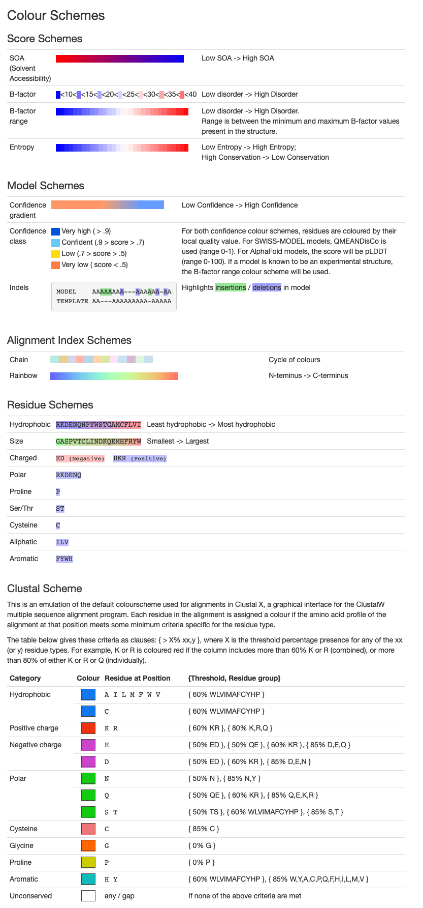
Color scheme explanations taken from: https://swissmodel.expasy.org/docs/help
Except for a list of templates, one can find their Quaternary structure, Sequence Similarity comparison and Alignment of Selected Templates tabs on the top.
The Quaternary Structure view show clustered templates according to their oligomeric state, stoichiometry, topology and interface similarity.
Protein–protein interaction (PPI) Fingerprint shows how conserved residues are on the protein interfaces compared to the surface residues interacting with the solvent. This is naturally calculated only for templates in oligomeric states. A negative value of interface conservation (y-axis) indicates that interface residues are more conserved compared to surface residues. This estimate of conservation is derived from a multiple sequence alignment of homologous proteins using different identity cut-offs (x-axis). The interface conservation can be quite useful in defining how well template interfaces adapt to the target protein family. Thus, the closes homologues should reach the lowest interface conservation values in the highest possible identity cut-off.
Which template(s) show the evolutionary most conserved interface? Is this good?
In the Sequence Similarity plot, templates are clustered by their sequence identity and are represented by circles. Thus, templates with high sequence identity form clusters further away from clusters of lower sequence identity. The distance between templates is proportional to the sequence identity between them. You can see the name and the structure of each template by hovering over with your mouse.
If one selects multiple templates by checking the window in the Templates tab, their sequence alignment is shown in Alignment of Selected Templates.
By clicking on the More button, one can see the complete list of templates not shown in this preview, download the Template Search Log or PDB structures of selected templates.
Tip: Select templates of varying quality and coverage now and compare models made from them in the following step.
4. Model building
This step might take a bit longer than previous steps, since we are actually creating new models. To build a model from a selected template, first the identical atom coordinates are transferred, insertions and non-conserved amino acid sidechains are modelled in. This step is performed by the ProMod3 modelling engine which is based on the OpenStructure computational structural biology framework. ProMod3 extracts structural information from an aligned template structure in Cartesian space and if no suitable fragments are found, Monte Carlo sampling is employed to perform a conformational space search. The new sidechain conformations, which cannot be found in the template, are modelled based on the backbone dependent rotamer library. In the final stage, small structural distortions or steric clashes are resolved by a short energy minimization using the CHARMM27 forcefield.
5. Model estimation
Similarly as in Template selection, the list of built models is shown in Model Results. After clicking on individual models, you can examine their quality in multiple ways and plots next to seeing their 3D structure in the NGL viewer on the right.
GMQE (Global Model Quality Estimation) is expressed as a number between 0 and 1, reflecting the expected accuracy of a model built with that alignment and template, normalized by the coverage of the target sequence. Higher numbers indicate higher reliability. GMQE contains also QMEAN predictions, to increase reliability of the quality estimation.
The Global Quality Estimate consists of four individual terms: Cβ atoms only, all atoms, the solvation potential and the torsion angle potential. Here again, the lower values indicate that the models scores lower than the experimental structure (red) and higher values indicate, that the model scores higher than the experimental structure (blue).
SWISS-MODEL uses another method QMEAN to estimate the quality of freshly built models. QMEAN quantifies model accuracy as well as modelling errors per residue and globally - for the entire model. This is done using statistical potentials of mean force.
The QMEAN Z-score or the normalized QMEAN score shows the “degree of nativeness”, which indicates how the model is comparable to an experimental structure of similar size. QMEAN Z-score around 0 indicates good agreement, while score below -4.0 are given to models of low quality. This is also turned into the “thumbs-up” or “thumbs-down” symbol next to the QMEAN value.
QMEAN score per residue is shown in the Local Quality Estimate plot. The QMEANDisCo method is used in this step. QMEANDisCo compares interatomic distances in the model with ensemble information extracted from experimentally determined protein structures of target sequence homologues. The score shows similarity of the residues to the experimental structure and if it drops below 0.6, modelled residues are in general of low quality. Different chains are shown in different colours and the residue modelling-quality can be viewed in 3D by selecting Confidence (gradient) as the coloring method in the NGL viewer.
The comparison plot shows the QMEAN score of our model (red star) within all QMEAN scores of experimentally determined structures compared to their size (number of residues). Here the Z-score is equivalent to the standard deviation of the mean.
One can superimpose selected models by clicking on their 3D structure image and they appear in the NGL viewer. Very handy is the sequence coverage comparison which appears under the 3D structure view. Here the target sequence is in green, while the model sequences in blue.
For more detailed structure information, one can click on the Structure Assessment button. This feature can be used also as a separate interface https://swissmodel.expasy.org/assess where one can upload their PDB structure and this will be assessed.
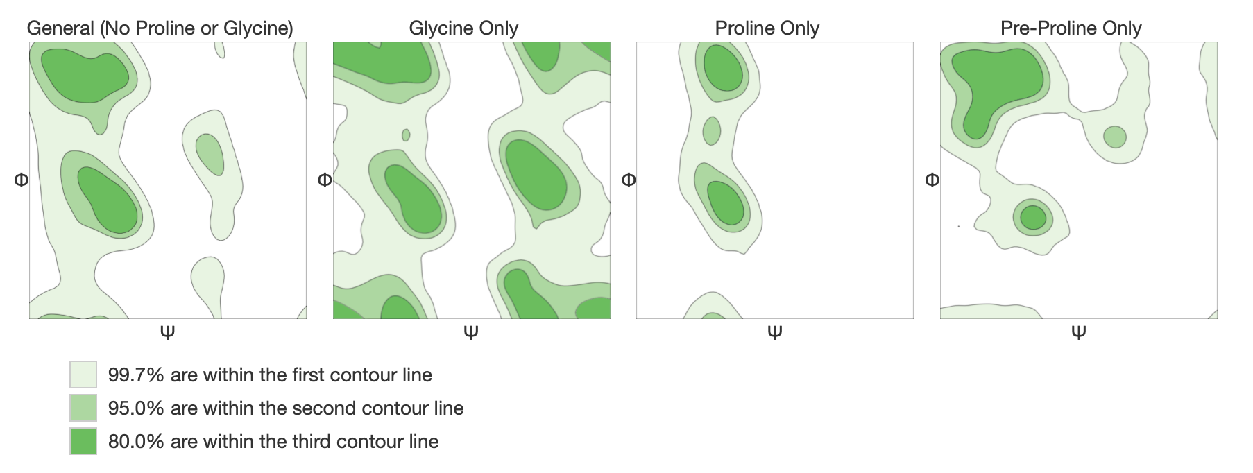
A Ramachandran plot is a way to visualize backbone dihedral angles of amino acid residues in the model against energetically favored regions of dihedrals of amino acids in general. These favored regions were obtained from more than 12000 experimental structures from PISCES. Moreover the model is validated by Molprobity both locally and globally. The quality of the structure is then expressed in Molprobity score, which should be as low as possible, and the percentage of Ramachandran Favoured residues, ideally above 98%. Clash score, outliers and bad angles and bonds should be as well as low as possible. More about structure assessment can be found in its documentation. Examples of Ramachandran plots for all residues below:
SWISS-MODEL offers a comprehensive overview of selected models, which can be open in a separate window.
On this page we see the list of models, the Consistency with Ensemble plot, the Ensemble Variance plot and superposed 3D structures of the models. In this case the ensemble represents the ensemble of selected models, thus consistency doesn’t indicate local quality of the model, but how consistent the residue quality is within the ensemble of models. Red color in both the Ensemble variance plot and in the 3D overlay shows higher differences of this region between models. If one aims to see the local quality of the model calculated with QMEAN, choose the QMEAN coloring method as in the example below:
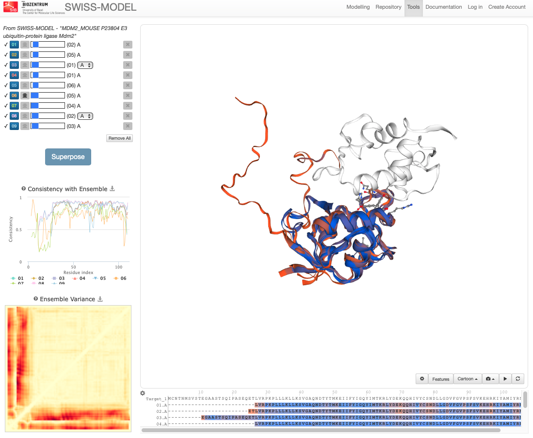
Notice how the selected residues are highlighted simultaneously in all plots, i.e. if you point at the Consistency with Ensemble plot, you will see where the given residue is in the sequence as well as in the 3D structure. The lower the consistency value, the more flexible the region is. This can be a good tool to quickly evaluate which model is the most stable one and which regions to take into account for further modelling. The default coloring scheme in the molecular viewer is consistency, or local deviations of a protein from the ‘consensus’ extracted from other selected models.
The Ensemble variance assesses the consistency of interatomic distances in the full ensemble. Only distances up to \(15Å\) are considered to reduce the effect of domain movement events.
Note that all figures can be downloaded by clicking on the Download icon. More information about the comparison page can be found on https://swissmodel.expasy.org/comparison/help.
When performing docking, we want to make sure that we only work with the relevant parts of the protein, i.e. the parts necessary for interactions. In some cases unstructured termini that are not vital for the complex formation might actually hinder the formation of a proper interface.
Except for downloading the model in the PDB format, one can also download a report that summarizes results for all models, suggest relevant publications and lists all possible templates. This is very useful to keep, however plain copy-pasting to your end report is strongly discouraged. Rather inspect all obtained results and select the relevant information and figures.
Congratulations!
You started with a sequence of a protein and went all the way from finding possible templates, to evaluating which to use, to building several models, assessing their quality, and finally selecting one representative. This model can now be used to offer insights on the binding of MDM2 to p53, or on the structure of the mouse MDM2 protein, or to seed new computational analysis such as docking.
You might want to continue with the tutorial on molecular dynamics simulations!