HADDOCK2.2 manual

Analysis

The analysis of the docking results are performed after the semi-flexible simulated annealing step and after the explicit solvent refinement. A number of standard CNS analysis scripts are automatically run by HADDOCK and the results are placed in the analysis directory in runX/structures/it1 and runX/structures/it1/water, respectively. Some of the generated output files are parsed automatically by HADDOCK to generate for example violations statistics (see violation analysis). Another important step consists in a manual analysis of the generated structures and their clusters. This is the critical step for the classification of the docking solutions and the identification of the best(s) cluster(s).

Topics:

Standard analysis performed by HADDOCK
Violation analysis
Manual analysis
Rerunning the analysis for a given cluster

Standard analysis performed by HADDOCK

The following CNS analysis scripts are automatically run by HADDOCK:

Average structure and RMSDs
Pairwise RMSD matrix
Energy and buried surface area analysis
Desolvation energy analysis
Per-residue interaction energy
Covalent geometry analysis
Distance restraints (AIRs, unambig, Hbonds) violations analysis
Dihedral angle restraints violations analysis
Residual dipolar coupling restraints violations analysis
Intervector projection angle restraints violations analysis
Diffusion anisotropy restraints violations analysis
Intermolecular hydrogen bonds analysis
Intermolecular hydrophobic contacts analysis

get_average.inp: This script will calculate an average structure by superimposing the structures on the backbone atoms of the flexible interface defined in the run.cns parameter file.

Note1:

The structures are fitted onto the average structures and written to disk in the analysis directory. Various average rmsds calculated over the ensemble of structure and rmsds from the average for each structure are output to file.

Output files:

fileroot_ave.pdb: average structure
filerootfit_1.pdb, filerootfit_2.pdb, ...: superimposed structures

Note2: The numbering of the superimposed PDB files does not correspond with the numbering in the it1 or water directories, but to the position of the structure in the sorted file.list file, i.e. structure number 1 in the analysis directory is the first (best) in file.list and structure number 50 is at position 50 in that file.
rmsave.disp: contains the RMSD from the average structure for each structure and the average values over the ensemble. For this, the structures are superimposed on the backbone atoms of the flexible interface (see Note1 above) and the following average RMSD values from the average structure are calculated and written to file:
- RMSD backbone interface of all molecules
- RMSD complete backbone of all molecules
- backbone interface of molecule A
- backbone interface of molecule B
- backbone interface of molecule C
- ...
In addition to the average RMSD calculated from the entire ensemble, the corresponding single structure RMSD values are listed in rmsave.disp
rmsdseq.disp: per residue RMSDs (backbone heavy atoms (N,CA,C), extended backbone heavy atoms (N,CA,CB,C,O), side-chain heavy atoms and all heavy atoms.
fileroot-reduced.crd: trajectory file containing only the coordinates of the flexible interface backbone atoms (see Note1 above); this reduced file is used to calculate the pairwise RMSD matrix and thereby speed up the calculations.

rmsd.inp: This script calculates the pairwise RMSD matrix over all structures. For this the structures are first superimposed on the flexible interface backbone atoms of molecule A and the RMSD is calculated on the flexible interface backbone atoms of the other molecules (see Note1 above). This RMSD can be termed: "ligand interface RMSD".

Output files:

fileroot_rmsd.disp: this file contains the pairwise RMSD matrix with on each line three number: the structure numbers of the two structures being compared and the corresponding RMSD value.

Note5: The numbering of the structures corresponds to the position of the structure in the sorted file.list file.

This file is used as input for the RMSD clustering.

energy.inp: this script performs the analysis of bonded and non-bonded energies per structure and averaged over the ensemble. Various energy terms are calculated:

over the entire complex
over the flexible interface only (as defined in the run.cns parameter file)
only the intermolecular energies (vdw and elec)

In addition, the buried surface area is also reported. The buried surface area is calculated by taking the difference between the sum of the solvent accessible surface area for each molecule separately and the solvent accessible area of the complex. The solvent accessible area is calculated using a 1.4A water probe radius and an accuracy of 0.075A (in case of memory problems for very large complexes increase this value, e.g. 0.1 or higher).

Output files:

energies.disp: this file contains the various energy terms per structure and averaged over the ensemble
- Complex statistics: Etot, Ebond, Eangle, Eimpr, Edihed, Evdw, Eelec
- Flexible interface statistics: Etot, Evdw, Eelec
- Intermolecular statistics: Etot, Evdw, Eelec
- Buried surface area

edesolv.inp: this script performs the analysis desolvation energy per structure and averaged over the ensemble. The desolvation energy is calculated using the empirical atomic solvation parameters from Fernandez-Recio et al. JMB 335:843 (2004). These are defined in the def_solv_param.cns CNS script in the protocols directory.

Output files:

edesolv.disp: this file contains the desolvation energy per structure and averaged over the ensemble

ene-residue.inp: this script performs a per-residue intermolecular interaction energy analysis for all residues which make intermolecular contacts. A residue is selected for analysis if it makes at least one contact within 5A within the ensemble analysed. Van der Waals, electrostatic and total interaction energies are reported per structure and as averages over the ensemble. They are calculated using the default 8.5A cutoff and a dielectric constant of 1 (all defined in the read_struc.cns CNS script.

Output files:

ene-residue.disp: this file contains the various energy terms per structure and averaged over the ensemble

Example:

    #Residue ASP 38 A - intermolecular energies
    #file Etot Evdw Eelec
    # PREVIT:e2a-hpr_161.pdb -16.7601 -3.41526 -13.3448
    # PREVIT:e2a-hpr_189.pdb -42.4061 -1.83788 -40.5682
    ...
    # mean values for interaction with residue ASP 38 A
    # ASP 38 A : Etot   -34.528 (+/- 21.4012 ) [kcal/Mol]
    # ASP 38 A : Evdw   -1.34906 (+/- 0.967306 ) [kcal/Mol]
    # ASP 38 A : Eelec  -33.179 (+/- 21.1375 ) [kcal/Mol]
    ...

The average per-residue values can be easily extracted from this file and sorted in decreasing contribution with the following command:

grep ": Evdw" ene-residue.disp |sort -gk7
grep ": Eele" ene-residue.disp |sort -gk7
grep ": Etot" ene-residue.disp |sort -gk7

print_geom.inp: this script performs the analysis of the covalent geometry, reporting on the deviations from ideal values for bonds, angles, impropers and dihedrals. The deviations per structure and averaged over the ensemble are reported.

Output files:

geom.disp: this file contains the averaged deviations from ideal geometry per structure and averaged over the ensemble.
print_geom.out: this file contains the listing of covalent terms deviating from the ideal geometry:
- bonds > 0.025 A
- angles > 2.5 degrees
- improper dihedrals > 2.5 degrees
- dihedral angles > 30 degrees

print_noes.inp: this script performs the analysis of distance (including AIR) restraint violations, generating output for all restraints combined and for each type of restraints (unambiguous, ambiguous (or AIRs) and hbonds) separately.

Output files:

noe.disp: this file contains the number of distance restraints violations per structure and averaged over the ensemble over all distance restraint classes and for each class (unambiguous, ambiguous, hbonds) separately. Distance restraints violation > 0.5, 0.3 and 0.1 A are reported.
print_dist_all.out: this file contains the violation listing for all distance restraints including hbond restraints.
print_dist_noe.out: this file contains the violation listing for all distance distance restraints (unambiguous and ambiguous classes).
print_noe_unambig.out: this file contains the violation listing for the unambiguous distance restraints.
print_noe_ambig.out: this file contains the violation listing for the ambiguous distance restraints (typically the class used to define Ambiguous Interaction Restraints).
print_dist_hbonds.out: this file contains the violation listing for the hydrogen bond distance restraints.

print_dih.inp: this script performs the analysis of dihedral angle restraint violations, listing per structure the violations above 5 degree and the average violations over the entire ensemble.

Output files:

dihedrals.disp: this file contains the number of dihedral restraints violations per structure and averaged over the ensemble.
print_dih.out: this file contains the violation listing for all dihedral restraints. This file is parsed automatically by HADDOCK to generate statistics on a restraint basis over all structures in the ensemble using the ana_dihed_viol.csh script provided in the tools directory (see violation analysis).

print_sani.inp: this script performs the analysis of dipolar coupling restraint violations, listing per structure the average rms violations and the number of violations above 1.0, 0.5 and 0.2 Hz, respectively. It also reports the average rms violation over the entire ensemble.

Output files:

sani.disp: this file contains the number of dipolar coupling violations per structure and averaged over the ensemble.
print_sani.out: this file contains the dipolar couplings violation listing. (No automatic parsing of this file is currently implemented).

print_vean.inp: this script performs the analysis of intervector projection angle restraint violations, listing per structure the violations above 5 degrees. It also reports the average rms violation over the entire ensemble.

Output files:

vean.disp: this file contains the number of intervector projection angle restraints violations per structure and averaged over the ensemble.
print_vean.out: this file contains the intervector projection angle restraints violation listing. (No automatic parsing of this file is currently implemented).

print_dani.inp: this script performs the analysis of diffusion anisotropy restraint violations, listing per structure the average rms violations and the number of violations above 1.0, 0.5 and 0.2, respectively. It also reports the average rms violation over the entire ensemble.

Output files:

dani.disp: this file contains the number of diffision anisotropy violations per structure and averaged over the ensemble.
print_dani.out: this file contains the diffision anisotropy violation listing. (No automatic parsing of this file is currently implemented).

print_hbonds.inp: this script performs the analysis of intermolecular hydrogen bonds. The definition of an hydrogen bond is however a crude one since it is only based on the proton-acceptor distance. This distance can be specified in the run.cns parameter file (default is 2.5A).

Output files:

hbonds.disp: this file contains a listing of all intermolecular hydrogen bonds over the ensemble of structures. It is automatically parsed by HADDOCK using the ana_hbonds.csh script located in the tools directory. This scripts generate a listing (ana_hbonds.lis) of intermolecular hydrogen bonds including the number of occurrences and the average hydrogen bond distance.

          ./ana_hbonds.csh hbonds.disp

print_nb.inp: this script performs the analysis of intermolecular hydrophobic contacts. An hydrophobic contact is identified when two carbon atoms are at less than a user-defined distance, typically 3.9A. This distance cut-off can be specified in the run.cns parameter file (default is 3.9A).

Output files:

nbcontacts.disp: this file contains a listing of all intermolecular hydrophobic contacts over the ensemble of structures. It is automatically parsed by HADDOCK using the ana_hbonds.csh script located in the tools directory. This scripts generate a listing (ana_nbconbtacts.lis) of intermolecular hydrophobic contacts including the number of occurrences and the average C-C distance.

          ./ana_hbonds.csh nbcontacts.disp

Violations analysis

HADDOCK performs automatically a number of violations analysis, generating a listing of violations including the number of times a restraint is violated and the average distance and violation per restraint. This is done for distance restraints (all distances (distances + Hbonds), distances only, unambiguous distances only, ambiguous distances only, dihedral angle restraints). A number of .lis files are generated in the analysis directory:

ana_dihed_viol.lis: dihedral angles violations if a dihedral file has been input in the new.html
ana_dist_viol.lis: all distance (including Hbonds) restraints violations
ana_hbond_viol.lis: hydrogen bond restraints violations
ana_noe_viol_all.lis: all distance restraints violations
ana_noe_viol_unambig.lis: unambiguous distance restraint violations
ana_noe_viol_ambig.lis: ambiguous distance restraints (this is the restraint type typically used for the ambiguous interaction restraints (AIRs).

Distance restraint violations > 0.3 A and dihedral angle restraints violations > 5 degree are reported. All atoms belonging to one restraints are listed, which in the case of ambiguous interaction restraints can be a very large number exceeding 1000! A new line always starts with Rexp=.

Example:

 
    Rexp=   2.000 Rave=   4.739 Viol=  -2.739 #viol=  200 (    B    36   HIS     N ...
    Rexp=   2.000 Rave=   4.626 Viol=  -2.626 #viol=  200 (    B    65   ASP     N ...
    Rexp=   2.000 Rave=   4.345 Viol=  -2.345 #viol=  200 (    B    33   GLN     N ...
    Rexp=   2.000 Rave=   4.037 Viol=  -2.037 #viol=    1 (    B    92   GLY     N ...
    Rexp=   2.000 Rave=   3.225 Viol=  -1.225 #viol=   63 (    A    37   SER     N ...
    ...

Rexp= 2.000 corresponds to the upper distance restraint (in Angstrom) defined in the AIR restraint file).

Rave= 4.739 corresponds to the average distance (in Angstrom) in the calculated structures.

Viol= -2.739 corresponds to the violation in Angstrom.

#viol= 200 corresponds to the number of structures in which the restraint is violated.

Manual analysis

An important part of the analysis, namely the analysis of the clusters, needs to be performed manually. A number of scripts are provided for this purpose in the runX/tools directory.

ana_structures.csh: This script should run once the file.list file has been created. It extracts from the header of the PDB files various energy terms, violation statistics and buried surface area and calculates the RMSD of each structure compared to the lowest energy one (if the location of ProFit is defined (see installation and software links)).

To run it type:

   $HADDOCKTOOLS/ana_structures.csh

in the directory where file.list has been created (e.g. structures/it1 or structures/it1/water).

Ten files are created:

structures_haddock-sorted.stat
structures_air-sorted.stat
structures_airviol-sorted.stat
structures_bsa-sorted.stat
structures_dH-sorted.stat
structures_Edesolv-sorted.stat
structures_ene-sorted.stat
structures_nb-sorted.stat
structures_nbw-sorted.stat
structures_rmsd-sorted.stat

These files looks like:

 
#struc haddock-score RMSD-Emin Einter Enb Evdw+0.1Eelec Evdw Eelec Eair Ecdih Ecoup Esani Evean Edani #NOEviol #Dihedviol #Jviol #Saniviol #veanviol #Daniviol bsa dH Edesolv
e2a-hpr_71w.pdb -164.13017 0.000 -629.446 -635.908 -107.853 -49.1804 -586.728 6.4629 0 0 0 0 0 0 0 0 0 0 0 1613.82 -8593.04 1.74954
e2a-hpr_171w.pdb -156.04058 0.748 -613.411 -624.683 -103.675 -45.7858 -578.897 11.2722 0 0 0 0 0 0 0 0 0 0 0 1663.99 -8501.99 4.3974
e2a-hpr_38w.pdb -150.756688 0.624 -574.337 -587.378 -97.1234 -42.6507 -544.727 13.0407 0 0 0 0 0 0 0 0 0 0 0 1688.07 -8600.72 -0.464658
...

The first line of those files gives the description of the columns, e.g. the first column corresponds to the pdb file, the second column to the combined HADDOCK score, the third to the backbone RMSD from the lowest energy structure, the third column to the total intermolecular energy (sum of all energy terms), the fourth column to the intermolecular non-bonded energy (vdw+elec),...

You can generated a plot of the HADDOCK score as a function of the RMSD (using XMGR for example).

A simple script called make_ene-rmsd_graph.csh is provided in $HADDOCKTOOLS which allows you to generate an input file for Xmgr/XmGrace. Simply specify two columns to extract data from and a filename:

  $HADDOCKTOOLS/make_ene-rmsd_graph.csh 3 2 structures_unsorted.stat

This will generate a file called ene_rmsd.xmgr which you can display with xmgr or xmgrace:

  xmgrace ene_rmsd.xmgr

RMSD-based clustering of solutions using cluster_struc: The clustering is run automatically by HADDOCK in it1/analysis and it1/water/analysis based on the criteria defined in the run.cns file. In case RMSD-based clustering has been selected, a reasonable cutoff value to start with for protein-protein complexes is 7.5A. We recommend however that you try using different cut-offs for the clustering since it is difficult to know a priori the best cut-off. This will depend on the system under study and the number of experimental restraints used to drive the docking. If only a small fraction of the structures cluster, try increasing the cut-off.

cluster_struc is a simple C++ program provided in the tools directory that read the fileroot_rmsd.disp file containing the pairwise rmsd matrix and generates clusters. This program should have been compiled for your system during installation.

Two clustering algorithms are implemented:

using an algorithm as described in Daura et al. Angew. Chem. Int. Ed. 38:236-240 (1999): count number of neighbors using cut-off, take structure with largest number of neighbors with all its neighbors as cluster and eliminate it from the pool of clusters. Repeat for remaining structures in pool.
full linkage: add a structure to a cluster when its distance to any element of the cluster is less than the cutoff.

The full linkage option generates thus larger clusters and the structures within a cluster can thus differ more. It is called by using the -f option. The default option used by HADDOCK is the first one (algorithm of Daura et al.). To use full linkage rerun the clustering manually.

The usage is:

 
   cluster_struc [-f]  fileroot_rmsd.disp cut-off  min_cluster_size >cluster.out

Example for its use:

 
  cluster_struc e2a-hpr_rmsd.disp 7.5 4 >cluster.out

will create clusters using a 7.5 A RMSD cut-off requiring a minimum of four structures per cluster.

The output looks like:

    Cluster 1 -> 8 1 2 3 5 6 7 9 10 11 12 13 14 15 ...
    Cluster 2 -> 23 25 26 29 39 62 66 67 72 74 78 ...
    Cluster 3 -> 153 4 32 43 96 131 147 158 163 ..

The numbers correspond to the structure number in the analysis file. For example 8 corresponds to structure number 8 in analysis, i.e, the eigth structure in file.list in it1/water. The first structure of each cluster above corresponds to the cluster center. The remaining structures are sorted according to their index.

Contact-based clustering of solutions using cluster_fcc.py: The clustering is run automatically by HADDOCK in it1/analysis and it1/water/analysis based on the criteria defined in the run.cns file. In case FCC clustering has been chosen (which means clustering based on the fraction of common contacts), a reasonable cutoff value to start with for protein-protein complexes is 0.75. We recommend however that you try using different cut-offs for the clustering since it is difficult to know a priori the best cut-off. This will depend on the system under study and the number of experimental restraints used to drive the docking. If only a small fraction of the structures cluster, try decreasing the cut-off.

cluster_fcc.py is a python code provided in the tools directory that read the fileroot_fcc.disp file containing the pairwise fraction of common contact matrix and generates clusters. The clustering algorithm is described in Rodrigues et al. Proteins: Struc. Funct. & Bioinformatic, 80 1810-1817 (2012).

The usage is:

 
Usage: cluster_fcc.py   [options]

Options:
  -h, --help            show this help message and exit
  -o OUTPUT_HANDLE, --output=OUTPUT_HANDLE
                        Output File [STDOUT]
  -c CLUS_SIZE, --cluster-size=CLUS_SIZE
                        Minimum number of elements in a cluster [4]

Example for its use:

 
  python cluster_fcc.py e2a-hpr_fcc.disp 0.75 -c 4 >cluster.out

will create clusters using a 0.75 FCC cut-off requiring a minimum of four structures per cluster.

The output looks the same as for the RMSD-based clustering explained above

ana_clusters.csh: This script takes the output of cluster_struc to perform an analysis of the various clusters, calculating average energies, RMSDs and buried surface area per cluster.

To run it, type with as argument the output file of the clustering, e.g.:

   $HADDOCKTOOLS/ana_clusters.csh [-best #] analysis/cluster.out

The [-best #] is an optional (but recommended!) argument to generate additional files with cluster averages calculated only on the best # structures of a cluster. The best structures are selected based on the HADDOCK score defined in run.cns, i.e. the sorting found in file.list. This allows to remove the dependency of the cluster averages upon the size of the respective clusters. The following example will calculate cluster averages over the best 45 structures.

   $HADDOCKTOOLS/ana_clusters.csh -best 4 analysis/cluster.out

The ana_clusters.csh script analyzes the clusters in a similar way as the ana_structures.csh script, but in addition generates average values over the structures belonging to one cluster. It creates a number of files for each cluster containing the cluster number clustX in the name:

file.cns_clustX
file.nam_clustX
file.list_clustX
And in addition if the option -best Y is used:
file.cns_clustX_bestY
file.nam_clustX_bestY
file.list_clustX_bestY
Note9: Those files can be used to repeat the HADDOCK analysis for a single cluster (see below).
file.nam_clustX_bsa
file.nam_clustX_dH
file.nam_clustX_Edesol
file.nam_clustX_ener
file.nam_clustX_haddock-score
file.nam_clustX_rmsd
file.nam_clustX_rmsd-Emin
file.nam_clustX_viol
Note10: The ordering of the structures in those files follows the HADDOCK score ranking.

Eight files containing various averages over clusters are created:

cluster_bsa.txt
cluster_dH.txt
cluster_Edesolv.txt
cluster_ener.txt
cluster_haddock.txt
cluster_rmsd.txt
cluster_rmsd-Emin.txt
cluster_viol.txt

and twelve files combining all the above information and sorted based on various criteria:

clusters_haddock-sorted.stat
clusters.stat
clusters_air-sorted.stat
clusters_bsa-sorted.stat
clusters_dani-sorted.stat
clusters_dH-sorted.stat
clusters_Edesolv-sorted.stat
clusters_ene-sorted.stat
clusters_nb-sorted.stat
clusters_nbw-sorted.stat
clusters_sani-sorted.stat
clusters_vean-sorted.stat

If the option -best is given with a number of structures, additional files with as extension _best# will be created containing the average values over the best # structures.

You can plot the HADDOCK score of the clusters as a function of their RMSD from the lowest energy structure (using xmgr/xmgrace for example).

graph

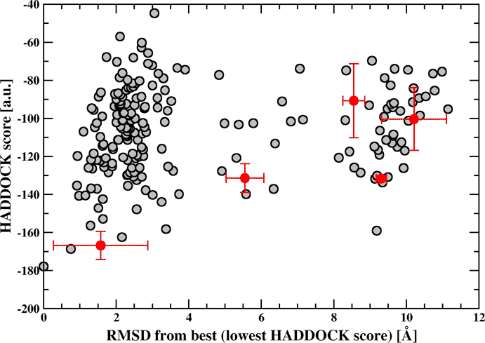
The gray circles correspond to the individual structures and the filled circles correspond to the cluster averages with the standard deviation indicated by bars.

The assumption is then that the best (lowest) HADDOCK score structures of the best (lowest) HADDOCK score cluster are the best solution generated by HADDOCK. It is then up to you to confirm that using any kind of information you can get such as for example:

mutagenesis data
conservation of given residues from multiple alignments
...

Rerunning the analysis for a given cluster

It is possible to rerun the HADDOCK analysis for a given cluster. For this, the file.cns, file.list and file.nam files should be renamed by adding for example a suffix _all. These three files contain the sorted list of all structures calculated. Similarly, the analysis directory should be renamed. Create then an empty analysis directory and cope the files containing the PDB file listings for a given cluster (these are created when performing the analysis of the clusters with ana_clusters.csh) to file.cns, file.list and file.nam, respectively.

To simplify this entire procedure, we are providing a csh script named make_links.csh in the tools directory (defined by the environment variable $HADDOCKTOOLS). To make the links type:

    $HADDOCKTOOLS/make_links.csh clust1

This will automatically move the original files (file.cns, file.list and file.nam) and rename the analysis directory. A new analysis directory called analysis_clust1 will be created and a link to it will be created as analysis. Similarly, links will be created for the three listing files:

   file.cns  -> file.cns_clust1
   file.list -> file.list_clust1
   file.nam  -> file.nam_clust1

To rerun the analysis go back to the runX directory and restart HADDOCK.

Warning: In case you wish to experiment with different clustering cut-offs restore first the original files containing the information for all calculated structures with the command:

   $HADDOCKTOOLS/make_links.csh all