

HADDOCK2.4 DNA-small molecule docking tutorial
This tutorial consists of the following sections:
- Introduction
- Requirements and Setup
- HADDOCK general concepts
- Inspecting and preparing the d(CGCAATTGCG) DNA helix for docking
- Preparing the Netropsin for docking
- Setting up the docking
- Analysing the results
- Visualization of the models and comparison with a reference structure
- Congratulations!
- Additional docking runs
Introduction
This tutorial will demonstrate the use of HADDOCK for ab-initio predicting the structure of a DNA-small molecule complex. Namely, we will dock the Netropsin and the DNA d(CGCAATTGCG). The Netropsin is a small molecule, first isolated from the actinobacterium Streptomyces, that exerts an antiviral and antibiotic activity. The Netropsin non-colvalently binds to DNA and prevent DNA replication and transcription by inhibiting polymerase reaction. Elucidating the binding mode of Netropsin with its target DNA sequences has helped developing candidate antibiotics and antitumor with similar mode of action. The d(GGCCAATTGG) structure in the free form have been determined using X-ray crystallography (PDB ID 252D). For this tutorial, we will predict the Netropsin/d(GGCCAATTGG) binding mode with no a-priori information on the nucleic acids involved in the interaction.
For this tutorial we will make use of the HADDOCK2.4 webserver.
- R.V. Honorato, M.E. Trellet, B. Jiménez-García1, J.J. Schaarschmidt, M. Giulini, V. Reys, P.I. Koukos, J.P.G.L.M. Rodrigues, E. Karaca, G.C.P. van Zundert, J. Roel-Touris, C.W. van Noort, Z. Jandová, A.S.J. Melquiond and A.M.J.J. Bonvin. The HADDOCK2.4 web server: A leap forward in integrative modelling of biomolecular complexes. Nature Prot., Advanced Online Publication DOI: 10.1038/s41596-024-01011-0 (2024).
Throughout the tutorial, coloured text will be used to refer to questions or instructions, and/or PyMOL commands.
This is a question prompt: try answering it! This an instruction prompt: follow it! This is a PyMOL prompt: write this in the PyMOL command line prompt!
Requirements and Setup
In order to run this tutorial you will need to have the following software installed: PyMOL.
Additionally, you will also need to run commands in a Unix-like terminal. If you are running this on a Mac or Linux system then
appropriate shells (all commands should work under bash) are already part of the system. Windows users might have to install additional software or activate the
Windows Subsystem for Linux. We consider this to be an advanced
tutorial made with a specific application of HADDOCK in mind. Thus, it assumes familiarity with HADDOCK as well as with the command line and scripting tools such as awk, sorted and grep.
All files, scripts and data for running this tutorial can be downloaded as a gzipped tar archive from here. Extract the archive in the directory where you want to run the tutorial with the following command:
tar xfz DNA-small-molecule.tgz
cd DNA-small-molecule
This will create a DNA-small-molecule directory where you will find various scripts and data.
Prior to getting started we need to setup our environment. The simplest way to do that would be to make use of anaconda.
If you are unfamiliar with anaconda/conda check the nice introduction by João Rodrigues.
Assuming an existing installation of anaconda, the following command should take care of all required python packages.
conda env create --file scripts/requirements.yml
conda activate haddock-shape-tutorial_env
After activating the environment we also need to install the pdb-tools package which can be achieved with the following command:
Also, if not provided with special workshop credentials to use the HADDOCK portal, make sure to register in order to be able to submit jobs. Use for this the following registration page: https://wenmr.science.uu.nl/auth/register/haddock.
HADDOCK general concepts
HADDOCK (see https://www.bonvinlab.org/software/haddock2.4/) is a collection of python scripts derived from ARIA (https://aria.pasteur.fr) that harness the power of CNS (Crystallography and NMR System – https://cns-online.org) for structure calculation of molecular complexes. What distinguishes HADDOCK from other docking software is its ability, inherited from CNS, to incorporate experimental data as restraints and use these to guide the docking process alongside traditional energetics and shape complementarity. Moreover, the intimate coupling with CNS endows HADDOCK with the ability to actually produce models of sufficient quality to be archived in the Protein Data Bank.
A central aspect to HADDOCK is the definition of Ambiguous Interaction Restraints or AIRs. These allow the translation of raw data such as NMR chemical shift perturbation or mutagenesis experiments into distance restraints that are incorporated in the energy function used in the calculations. AIRs are defined through a list of residues that fall under two categories: active and passive. Generally, active residues are those of central importance for the interaction, such as residues whose knockouts abolish the interaction or those where the chemical shift perturbation is higher. Throughout the simulation, these active residues are restrained to be part of the interface, if possible, otherwise incurring in a scoring penalty. Passive residues are those that contribute for the interaction, but are deemed of less importance. If such a residue does not belong in the interface there is no scoring penalty. Hence, a careful selection of which residues are active and which are passive is critical for the success of the docking. The docking protocol of HADDOCK was designed so that the molecules experience varying degrees of flexibility and different chemical environments, and it can be divided in three different stages, each with a defined goal and characteristics:
1. Randomization of orientations and rigid-body minimization (it0) In this initial stage, the interacting partners are treated as rigid bodies, meaning that all geometrical parameters such as bonds lengths, bond angles, and dihedral angles are frozen. The partners are separated in space and rotated randomly about their centres of mass. This is followed by a rigid body energy minimization step, where the partners are allowed to rotate and translate to optimize the interaction. The role of AIRs in this stage is of particular importance. Since they are included in the energy function being minimized, the resulting complexes will be biased towards them. For example, defining a very strict set of AIRs leads to a very narrow sampling of the conformational space, meaning that the generated poses will be very similar. Conversely, very sparse restraints (e.g. the entire surface of a partner) will result in very different solutions, displaying greater variability in the region of binding.
See animation of rigid-body minimization (it0):
2. Semi-flexible simulated annealing in torsion angle space (it1) The second stage of the docking protocol introduces flexibility to the interacting partners through a three-step molecular dynamics-based refinement in order to optimize interface packing. It is worth noting that flexibility in torsion angle space means that bond lengths and angles are still frozen. The interacting partners are first kept rigid and only their orientations are optimized. Flexibility is then introduced in the interface, which is automatically defined based on an analysis of intermolecular contacts within a 5Å cut-off. This allows different binding poses coming from it0 to have different flexible regions defined. Residues belonging to this interface region are then allowed to move their side-chains in a second refinement step. Finally, both backbone and side-chains of the flexible interface are granted freedom. The AIRs again play an important role at this stage since they might drive conformational changes.
See animation of semi-flexible simulated annealing (it1):
3. Refinement in Cartesian space (itw) Note:As a final step, a short energy minimisation is performed.
The performance of this protocol of course depends on the number of models generated at each step. Few models are less probable to capture the correct binding pose, while an exaggerated number will become computationally unreasonable. The standard HADDOCK protocol generates 1000 models in the rigid body minimization stage, and then refines the best 200 – regarding the energy function - in both it1 and water. Note, however, that while 1000 models are generated by default in it0, they are the result of five minimization trials and for each of these the 180º symmetrical solution is also sampled. Effectively, the 1000 models written to disk are thus the results of the sampling of 10.000 docking solutions.
The quality of the final models is evaluated by computing the root mean square deviation (RMSD) of the small molecule after superomposing the DNA strands of the docking model to the DNA strands of the reference structure. Herein, we make use of PROFit to superimpose the DNA structures and of the obrms module of OpenBabel to compute the symetry corrected RMSD of the small molecule.
Inspecting and preparing the d(CGCAATTGCG) DNA helix for docking
We will now inspect the DNA structure. For this start PyMOL and in the command line window of PyMOL (indicated by PyMOL>) type:
You should see a backbone representation of the DNA and the stick representation of the small molecule. As a preparation step before docking, it is advised to remove any water and other small molecules (e.g. small molecules from the crystallisation buffer), however do leave relevant co-factors if present. Herein, the PDB file contains water molecules and magnesium ions whose location may move upon small molecule. You can remove those in PyMOL by typing:
remove resn HOH remove name MG
Make sure that there is no atom associated to multiple occupancy. show lines
Do you obeserve multiple occupancy atoms ?
In this scenario, it is important to identify which of the multiple locations of the atom is the most observed in vitro. This information is provided in the PDB file into occupancy factor column (i.e. the column found after the XYZ coordinated and before the b-factor column).
To do so, first save the molecule as a new PDB file which we will call: 252d_ready.pdb
For this in the PyMOL menu on top select:
File -> Export molecule… Click on the save button Select as ouptut format PDB (*.pdb *.pdb.gz) Name your file 252d_ready.pdb and note its location
Read the PDB file to verify that column. cat 252d_ready.pdb
Do you observe double occupancy ?
If yes, keep the coordinates associated to the major occupancy for each duplicated atom. PS: You should observe no double occupancy in the 252d file, therefore the next line is not worth applying.
grep ATOM 252d_ready.pdb | pdb_selaltloc > t ; mv t 252d_ready.pdb
As a last step, we clean the PDB file to prepare the HADDOCK submission
Preparing the Netropsin for docking
We will now prepare the Netropsin for docking. To make sure the tutorial we are presenting here sticks as closely as possible to a real-life modelling scenario we will be generating conformers starting from the SMILES string of the Netropsin. For this, we will use RDKit along with a predefined set of parameters that govern the behaviour of the program during the conformer generation.
The script we will use can be found in scripts/generate_conformers.py.
Running it with the -h flag will list all possible options the script
can be called with. We will run it with the optimal options that were estabilished during the benchmarking of this protocol benchmark.
./scripts/generate_conformers.py -i data/netropsin.smi -p 3sr -c 50 -m -o conformers.pdb
The above command will create a conformers.pdb file in the current working directory.
We need to process the file to remove the redundant data in it and prepare it for docking.
grep -v CONECT conformers.pdb | sed -e 's/UNL/UNK/' | pdb_chain -B > t; mv t conformers.pdb
Open Pymol to observe the generated conformers How many conformers have been generated ?
Setting up the docking
For the docking we will use the new portal of HADDOCK2.4. If you are already
registered with HADDOCK or have been provided with course credential then you can proceed to job submission immediately.
Alternatively, you can request an account through the registration portal. Keep in mind that for this tutorial you will
have to request guru level access, this is done by selecting the Request Elevated Access in your user profile.
After logging in you are greeted with the first part of the submission portal. Make sure to use an informative name for the run.
-
Step1: Define a name for your docking run in the field “Job name”, e.g. DNA-small-molecule.
-
Step2: Select the number of molecules to dock. Since this is a two-body docking between the template receptor and the generated conformers so we should set the number of molecules to 2.
- Step3: Input the DNA PDB file. For this unfold the Molecule 1 - input if it isn’t already unfolded.
Molecule 1 - input -> PDB structure to submit -> Upload the file named 252d_ready.pdb
Molecule 1 - input -> Fix molecule at its original position during it0? -> True
- Step4: Input the ensemble of ligand conformations PDB file. For this unfold the Molecule 2 - input if it isn’t already unfolded.
Molecule 2 - input -> PDB structure to submit -> Upload the file named conformers.pdb
Molecule 2 - input -> What kind of molecule are you docking? -> Ligand
-
Step 5: Click on the “Next” button at the bottom left of the interface. This will upload the structures to the HADDOCK webserver where they will be processed and validated (checked for formatting errors). The server makes use of Molprobity to check side-chain conformations, eventually swap them (e.g. for asparagines) and define the protonation state of histidine residues.
-
Step 6: The second submission tab “Input Parameters” can be skipped entirely since we will be defining our restraints through tbl files instead of doing it through the interface. Click on “Next”.
-
Step 7: Define the center-of-mass restraints between the small molecule and the DNA and DNA restraints to maintain preserve its structure. For this unfold the Distance restraints menu if not already unfolded
For DNA/small molecule docking we advise to keep all hydrogen atoms (non-polar hydrogens are deleted by default by the server)
Distance restraints -> Create DNA/RNA restraints? -> True
Distance restraints -> Remove non-polar hydrogens? -> False
Distance restraints -> Use tight center of mass restraints? -> False
- Step 8: Change the sampling parameters. For this unfold the Sampling parameters menu if not already unfolded
Since we have 50 conformations in the ligand ensembles, change the number of models to generate to 1000 (20 per ligand conformation).
Sampling parameters -> Number of structures for rigid body docking -> 1000
Sampling parameters -> Sample 180 degrees rotated solutions during rigid body EM -> False
Sampling parameters -> Number of structures for semi-flexible refinement -> 400
For DNA/small molecule docking we do not recommend to perform the final refinement, but instead use the models from the semi-flexible refinement stage (it1).
Sampling parameters -> Perform final refinement? -> False
- Step 9: Change the interaction parameters. For this unfold the Energy and interaction parameter menu if not already unfolded
Energy and interaction parameter -> Epsilon constant for the electrostatic energy term in it0 -> 78
Energy and interaction parameter -> Epsilon constant for the electrostatic energy term in it1 -> 10
- Step 9: Change the scoring function. For this unfold the Scoring parameter menu if not already unfolded
Scoring parameters -> Evdw 1 -> 1.0
- Step 10: Change the advanced sampling parameters. For this unfold the Advanced sampling parameters menu if not already unfolded
Advanced Sampling Parameters -> Number of MD steps for rigid body high temperature TAD -> 0
Advanced Sampling Parameters -> Number of MD steps during first rigid body cooling stage -> 500
- Step 11: You are ready to dock! Click “Submit”. If everything went well your docking run has been added to the queue and might take anywhere from a few hours to a few days to finish depending on the load on our servers.
Note: that prior to submission you also have the option to download the processed data (in the form of a tgz archive) and a .json file which contains all the settings and input structures for our run. We strongly recommend to download this file as it will allow you to repeat the run by using the file upload inteface of the HADDOCK webserver. This .json file can serve as input reference for the run, and could be provided as supplementary material in a publication. This file can also be edited to change a few parameters for example.
The generated json file for this shape-based submission is provided at data/job_params.json.
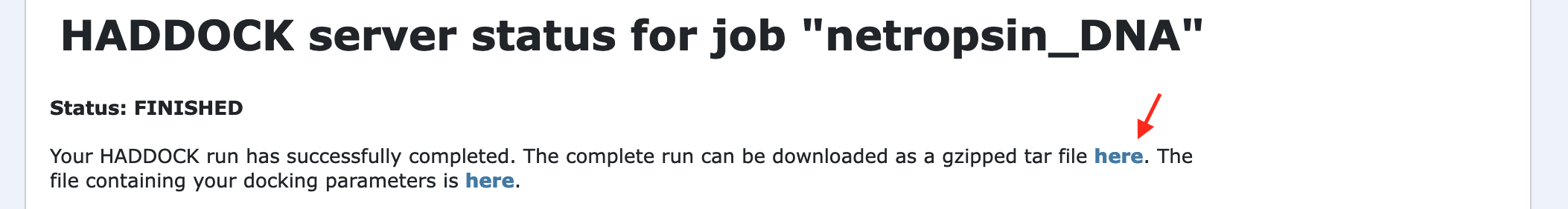
Upon submission you will be presented with a web page which also contains a link to the previously mentioned .json file as well as some information about the status of the run.
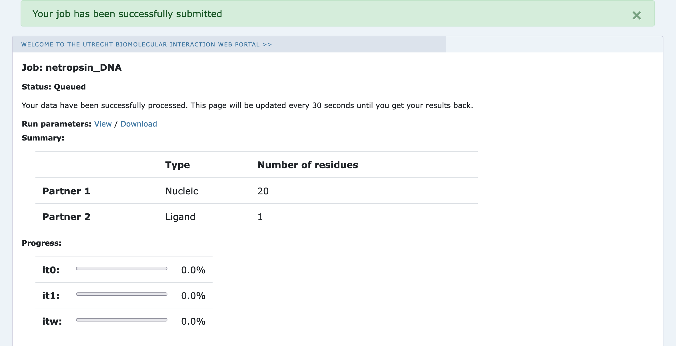
Currently your run should be queued but eventually its status will change to “Running”:
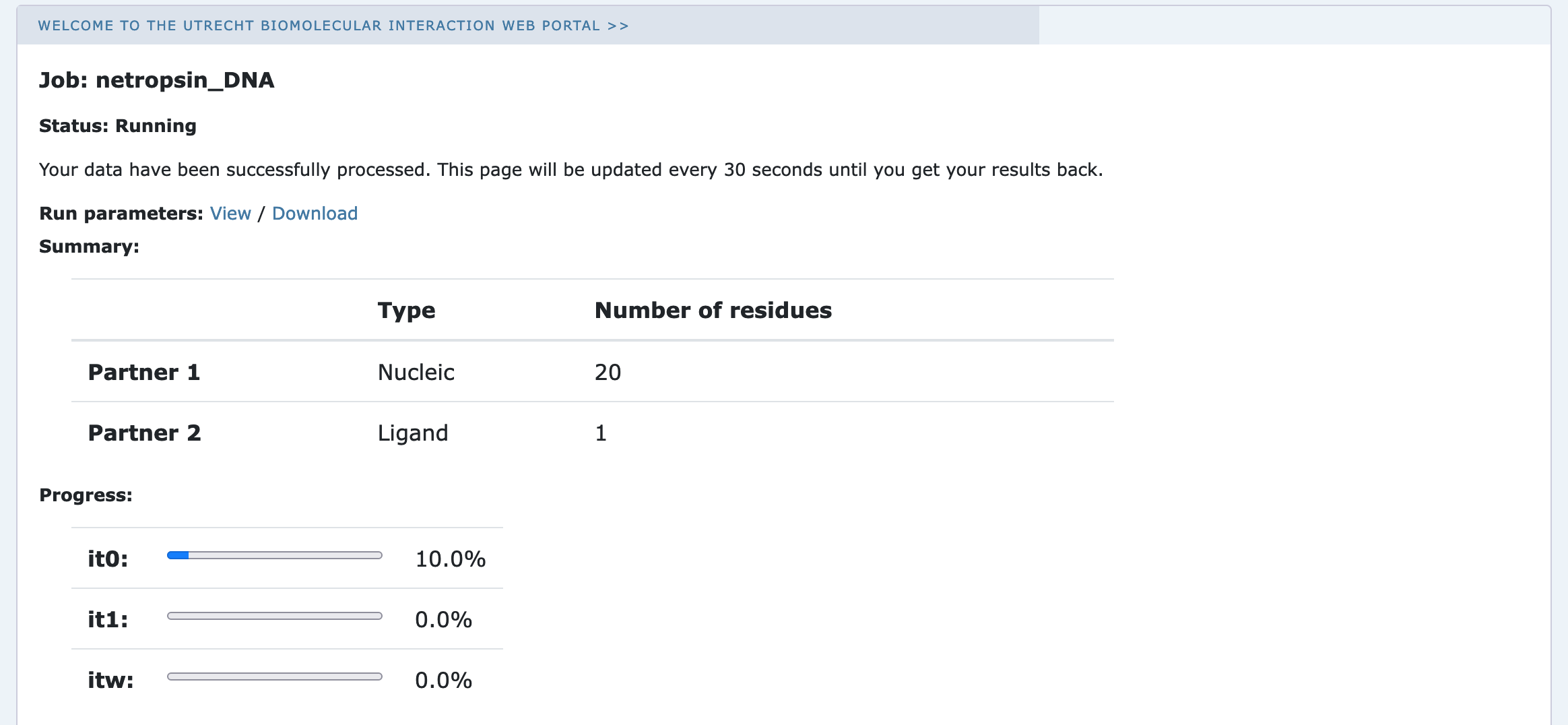
The page will automatically refresh and the results will appear upon completions (which can take between 1/2 hour to several hours depending on the size of your system and the load of the server). You will be notified by email once your job has successfully completed.
Analysing the results
Once your run has completed you will be presented with a result page showing the cluster statistics and some graphical representation of the data (and if registered, you will also be notified by email). Such an example output page can be found here in case you don’t want to wait for the results of your docking run.
How many clusters are generated?
Just glancing at the page tells us that our run has been a success both in terms of the actual run and the post-processing that follows every run. Examining the summary page reveals that in total HADDOCK only clustered 30 models in 7 different clusters, meaning that only 15% of the docking models have been considered for the analysis.
Note: The bottom of the page gives you some graphical representations of the results, showing the distribution of the solutions for various measures (HADDOCK score, van der Waals energy, …) as a function of the Fraction of Common Contact with- and RMSD from the best generated model (the best scoring model). The graphs are interactive and you can turn on and off specific clusters, but also zoom in on specific areas of the plot.
The bottom graphs show you the distribution of scores (Evdw, Eelec and Edesol) for the various clusters as a function of the Fraction of Common Contact (FCC) and also with interface-RMSD from the best scoring model. The graphs are interactive and you can turn on and off specific clusters (single structures in this case), but also zoom in on specific areas of the plot.
The ranking of the clusters is based on the average score of the top 4 members of each cluster. The HADDOCK score in this case corresponds to the it1 score (see for details the online manual pages). It is defined as:
HADDOCK-it1-score = 1.0 * Evdw + 1.0 * Eelec + 1.0 * Edesol + 0.1 * Eair - 0.01 * BSA
where Evdw is the intermolecular Van der Waals energy, Eelec the intermolecular electrostatic energy, Edesol represents an empirical desolvation energy term adapted from Fernandez-Recio et al. J. Mol. Biol. 2004, Eair the distance restraint energy and BSA the buried surface area in Å. The various components of the HADDOCK score are also reported for each cluster on the results web page.
PS: Top scoring models may not belong to a cluster and may be skipped in the analysis.
Download the full run available from the first link of the results page to have access to all the generated models. The structures/it1 folder contains the 400 final docking models and score details.
Consider the cluster scores and their standard deviations. Is the top ranked cluster significantly better than the second one? (This is also reflected in the z-score).
In case the scores of various clusters are within standard devatiation from each other, all should be considered as a valid solution for the docking. Ideally, some additional independent experimental information should be available to decide on the best solution. In this case we do have such a piece of information: the phosphate transfer mechanism (see Biological insights below).
Note: The type of calculations performed by HADDOCK does have some chaotic nature, meaning that you will only get exactly the same results if you are running on the same hardware, operating system and using the same executable. The HADDOCK server makes use of EGI/EOSC high throughput computing (HTC) resources to distribute the jobs over a wide grid of computers worldwide. As such, your results might look slightly different from what is presented in the example output page. That run was run on our local cluster. Small differences in scores are to be expected, but the overall picture should be consistent.
Visualization of the models and comparison with a reference structure
The new HADDOCK2.4 server integrates the NGL viewer which allows you to quickly visualize a specific structure. For that click on the “eye” icon next to a structure.
For a closer look at the top models we can use the link on results webpage just above the Cluster 1 line to download the top10 models,or simply click here.
Download and save to disk the top 4 models of each cluster (use the PDB format)
Using the following command expand the contents of the tgz archive in your working directory:
tar xfz 117436-netropsin_DNA_summary.tgz
This will result in the creation of 28 PDB files in the current working directory, corresponding to the top4 models
of each cluster. The files are named cluster*_*.pdb with model cluster2_1.pdb being the model with the overall best HADDOCK score.
Important: Please note that the cluster number is not its ranking but a measure of how populated it is. Cluster 1 will always contain the most models, but it might not be the top ranking cluster. The order on the results webpage corresponds to the ranking. Please check the HADDOCK Manual for more information.
With the following command we can load the 28 models into PyMOL along with the reference structure provided in the data directory for closer examination.
pymol data/261d.pdb cluster*.pdb
Once all files have been loaded, type in the PyMOL command window:
show cartoon show sticks, org rm resn HOH util.cbc hide lines
Let’s then superimpose all models on the reference structure:
This will align all clusters on the DNA (d(CGCAATTGCG)), maximizing the differences in the orientation of chain B (Netropsin).
Examine the various clusters. How does the orientation of Netropsin differ between them?
How well does the docked models overlap with the one of the reference (261d) structure?
Note: You can turn on and off a cluster by clicking on its name in the right panel of the PyMOL window.
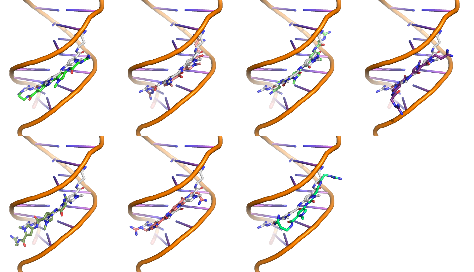
Superimposition of the best scoring pose of each cluster onto the reference complex (in white).
Is there a model that better overlaps with the reference structure?
What is the HADDOCK score of this model ?
Note: You can refer to the graphs at the bottom of the results summary page.
Observe which DNA-groove is targetted by the small molecule.
Is the small molecule a major- or minor-groove binder ?
Highlight the different nucleic acids.
set cartoon_ring_mode, 1 color palecyan, resn DA color lightpink, resn DT color lightblue, resn DC color paleyellow, resn DG
What DNA motif does the Netropsin bind to ? Cite the 4 main nucleic acids.
RMSD computation
As part of the analysis we can also compute the symmetry-corrected ligand RMSD for our model of choice. Before doing that we should make sure the models are aligned to the target. This can be done using for example the ProFit software.
If ProFit is installed in your system you can use the provided scripts/lzone to align a model to the target on the protein interface residues. The script will write the aligned file as tmp.pdb. For the top-scoring compound the commands to use are:
profit -f scripts/lzone ./data/261d.pdb cluster2_1.pdb grep UNK tmp.pdb | pdb_element > cluster2_ligand.pdb obrms ./data/261d_ligand.pdb cluster2_ligand.pdb
obrms (installed with Anaconda) reports a ligand RMSD value of 1.13 indicating excellent agreement between model and reference structures.
If you don’t have ProFit installed you can use instead PyMOL to fit the models on the binding site residues: Assuming you still have PyMOL open and have performed the above commands, do the following to fit the top model (cluster1) onto the binding site of the target:
select binding_site, resi 1:19 align cluster2_1 and backbone and binding_site, 261d and backbone and binding_site, cycles=0
Then save the aligned cluster2_1 by selecting from the PyMOL menu:
File -> Export molecule… Selection -> cluster2_1 Click on Save… Select as ouptut format PDB (*.pdb *.pdb.gz) Name your file tmp.pdb, note its location and move it to your working directory
You can then calculate the ligand RMSD with:
grep UNK tmp.pdb | pdb_element > tmp_ligand.pdb obrms ./data/261d_ligand.pdb tmp_ligand.pdb \rm tmp_ligand.pdb
Congratulations!
You have completed this tutorial. If you have any questions or suggestions, feel free to contact us via email or asking a question through our support center.
Additional docking runs
If you are curious and want learn more about HADDOCK and the impact of the input data on the docking results, consider performing and analysing, as described above, the following runs:
- Same run as above, but without defining the phosphorylated histidine
- Same run as above, but using only the first model of the HPR ensemble (edit the file to extract it)
And check also our education web page where you will find more tutorials!