

Protein-DNA docking Using HADDOCK High-Ambiguity Driven DOCKing
This tutorial consists of the following sections:
- Introduction
- Part I: Preparing the first HADDOCK2.4 docking run
- Part II: Preparing input structure files for the first HADDOCK run
- Part III: Understanding Ambiguous Interaction Restraints in Protein-DNA Docking
- Part IV: Analysing the results of first docking run
- Preparing the second HADDOCK run
Introduction
Structures of protein-DNA complexes fulfil a key role in our understanding of the complex regulatory mechanisms in the living cell. With the ever-increasing number of putative DNA-interacting proteins, there is a need for high-throughput structural biology pipelines.
However, not all biomolecular complexes are that straightforward to solve using experimental methods such as X-ray crystallography and Nucleic Magnetic Resonance (NMR) spectroscopy. Indeed, complexes that engage in transient interactions are, by definition, highly dynamic during interaction, while too big ones remain still a challenge for structural experimental techniques.
Computational methods for the calculation of structural models at atomic resolution have proven to be a valid toolset to help overcome some of these experimental limitations. Especially docking algorithms are becoming increasingly popular. These algorithms aim to solve the structure of a complex from its native constituents using various computational approaches. While very performant for protein-protein interactions, many of these algorithms suffer limitations when trying to model protein-DNA complexes such as the location of the interaction interfaces and dealing with conformational change upon complex formation.
This tutorial will introduce HADDOCK (High Ambiguity Driven DOCKing) [1] as a method to overcome some of the limitations associated with protein-DNA docking.
About this tutorial
This tutorial will introduce you to a practical approach for modelling protein-DNA complexes using HADDOCK2.4.
It is the advanced version of basic protein-DNA modelling tutorial which can be found in here.
You may therefore regard this tutorial as an extension of the introductory protein-DNA docking tutorial.
What is new in this tutorial?
This tutorial introduces the following theoretical and practical concepts of which many are unique for protein-DNA docking:
- Part I: Launch a protein-DNA docking run using HADDOCK2.4 webserver and provided starting structures.
- Part II: How to obtain DNA starting structures in various conformations suitable for use in HADDOCK? For this purpose, the 3D-DART web server is introduced.
- Part III: How to prepare Ambiguous Interaction Restraints (AIR) for protein-DNA docking? What information is available to construct AIRs? How to go about preparing AIRs in multi-body protein-DNA systems? How to make use of atom subsets in preparing restraints if there is sufficient information available?
- Part IV: Introduction to the dedicated AIR viewer plugin for the PyMol, that allows easy exploration and preparation of Ambiguous Interaction Restraints for HADDOCK.
- Part IV and V: How to perform an iterative protein-DNA docking run? How to use the 3D-DART web server to generate new models for a second docking run based on the results of the first docking run.
What are the main concepts introduced in this tutorial?
You will perform a docking of a protein-DNA system composed of 3 biomolecules (2 proteins and 1 DNA). All these molecules are in their unbound conformation. There are two major docking challenges you must deal with:
-
How to ensure that the docking is guided as such that the native interface between all three molecules is correctly modelled? You will use available biochemical and biophysical data to construct HADDOCK’s Ambiguous Interaction Restraints (AIRs) to deal with this. You will be introduced to the setup of specific restraints to guide the individual proteins to their respective operator half-sites and to use atom subsets in AIR generation to make use of the full potential of the available information.
-
How to ensure that all the molecules are allowed to change conformation at the interface to form the native complex? A special focus is on the DNA that often changes conformation globally upon interaction with a protein. This is expressed as DNA bending and twisting on a global scale and base pair as well as base pair step reorientations on a local scale.
You will also be introduced to the concept of 2-stage iterative docking [2,3] as a means of introducing large conformational changes that can occur in DNA. This approach is based upon the following principles:
- You start with an ideal double-stranded canonical DNA structure. At this stage there is no information available about the extent of conformational changes that might occur in the DNA.
- In the first docking run you will define nearly the full DNA as semi-flexible allowing it to change conformation upon interaction with the proteins.
- After the first docking you will analyse the conformation of the DNA in a selection of best docking solution looking for consistent trends in its global and local conformation. Does it for instance bend towards the protein or changes groove width?
- If consistent trends are found, you will use these to generate a new set of pre-bent and twisted DNA models. These models will hopefully have a conformation that resembles the bound conformation more closely and be freed of any helical distortions introduced during the docking.
- This ensemble of custom-built DNA models will be used in a second docking run.
Figure 1 shows an overview of the 2-stage protein-DNA docking procedure you will be using during this tutorial.
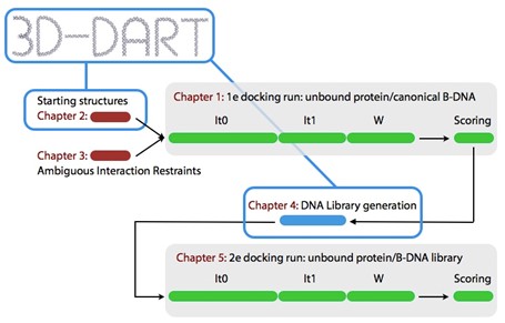
Figure 1: Overview of the 2-stage protein-DNA docking protocol followed in this tutorial. Every stage is discussed in its own part indicated in red.
Using this tutorial
You should be able to go through this tutorial in about 4 hours. Basic knowledge on the principles and use of HADDOCK is useful but not required. We will be using the HADDOCK 2.4 webserver https://wenmr.science.uu.nl/haddock2.4/ to perform the docking and the standalone version of HADDOCK to perform the analysis of the results.
- R.V. Honorato, M.E. Trellet, B. Jiménez-García, J.J. Schaarschmidt, M. Giulini, V. Reys, P.I. Koukos, J.P.G.L.M. Rodrigues, E. Karaca, G.C.P. van Zundert, J. Roel-Touris, C.W. van Noort, Z. Jandová, A.S.J. Melquiond and A.M.J.J. Bonvin The HADDOCK2.4 web server: A leap forward in integrative modelling of biomolecular complexes. Nature Protoc, 19, 3219–3241 DOI: 10.1038/s41596-024-01011-0 (2024)
Tutorial data set
In this tutorial you will perform a protein-DNA docking using the bacteriophage 434 Cro repressor protein and the OR1 operator as an example case. All the tutorial data are made available as a gzipped tar archive (.tgz) in the following address https://surfdrive.surf.nl/public.php/dav/files/CuyiqNVryeN2wNz.
Virtual Machine
This tutorial contains UNIX command line operations that should be done in a GNU/Linux operating system. If you do not have access to such type of OS, you can launch it in virtual environments that could be created by software such as VirtualBox or VMware. We recommend VirtualBox as the hypervisor and Ubuntu as the operating system, which is free to download and use, and is available at https://www.virtualbox.org/ and https://ubuntu.com/download/desktop. The complete installation guide of Ubuntu on the VirtualBox can be found in here.
Practical requirements
Running this tutorial requires several computational and knowledge pre-requisites:
- An active Internet connection is necessary to access the HADDOCK 2.4 web portal.
- The GNU/Linux operative system will be used for part 3 (Analysis). Simple knowledge in this OS would be helpful, but not necessary, namely folder navigation (cd) and editing of file contents (sed).
- ProFit http://www.bioinf.org.uk/software/profit/index.html will be used to perform superimposition of models and calculate various RMSD values.
- Pymol http://www.pymol.org will be used to visualize the structural models. Although most commands are listed and explained, basic working knowledge is advised.
Where can I find more information?
An elaborate discussion of all the concepts of protein-DNA docking and the various options of the HADDOCK docking software is beyond the scope of this tutorial. Where needed, some concepts will be explained throughout the tutorial to maintain the readability and flow of this tutorial. Every part end with a short ‘reference’ block that provides links to in depth literature or Internet documentation about various topics.
What if I do not find an answer to my questions? It is always possible that you have questions or run into problems for which you cannot find the answer in the regular documentation. Here are some additional links that you can find answers to your questions:
- Bioexcel user forum: https://ask.bioexcel.eu/c/haddock/6
- HADDOCK Help Center: https://wenmr.science.uu.nl/haddock2.4/help
- HADDOCK software and online manual: https://www.bonvinlab.org/software/haddock2.4/manual/
Tutorial icon conventions
Throughout the tutorial we will use the following special fonts and icons to perform certain tasks or draw your attention:
This is a question prompt: try answering it! This is an attention prompt: pay special attention to this! This an instruction prompt: follow it! This is a PyMOL prompt: write this in the PyMOL command line prompt! This is a Linux prompt: insert the commands in the terminal!
Introduction to the tutorial test case
To illustrate our protein-DNA docking protocol we will use as an example the complex between the bacteriophage 434 Cro repressor proteins and the OR1 operator.
Cro is part of the bacteriophage 434 genetic switch
Cro is a repressor protein of the temperate bacteriophage 434. It works in opposition to the phage’s repressor protein to control the genetic switch. The competition between both determines whether the phage embarks on a lytic or lysogenic lifecycle after infection. The repressors compete to gain control over an operator region containing three operators that determine the state of the lytic/lysogenic genetic switch. If Cro wins the late genes of the phage will be expressed and the result is lysis. If the phage repressor wins the transcription of Cro genes is further blocked and repressor synthesis is maintained, a state of lysogeny results.
Structure of the Cro-OR1 complex
The structure of bacteriophage 434 Cro in complex with the OR1 operator was solved by X-ray crystallography ([4], Figure 2). We will use this structure as reference (or target) during the remaining of the tutorial. Cro functions as a symmetrical dimer. Each subunit contains a helix-turn-helix (HTH) DNA binding motif. This is a typical DNA major groove-binding motif. Helices α2 and α3 are separated by a short turn. Helix α3 is the recognition helix that fits into the major groove of the operator DNA and is oriented with its axes parallel to the major groove. The side chains of each helix are thus positioned to interact with the edges of base pairs on the floor of the groove. Non-specific interactions also help anchor Cro to operator DNA. These include H-bonds between main chain NH groups and phosphate oxygens of the DNA in the region of the operator. Cro distorts the normal B-form DNA conformation: the OR1 DNA is bent (curved) by Cro, and the middle region of the operator is overwound, as reflected in the reduced distance between phosphate backbones in the minor groove.
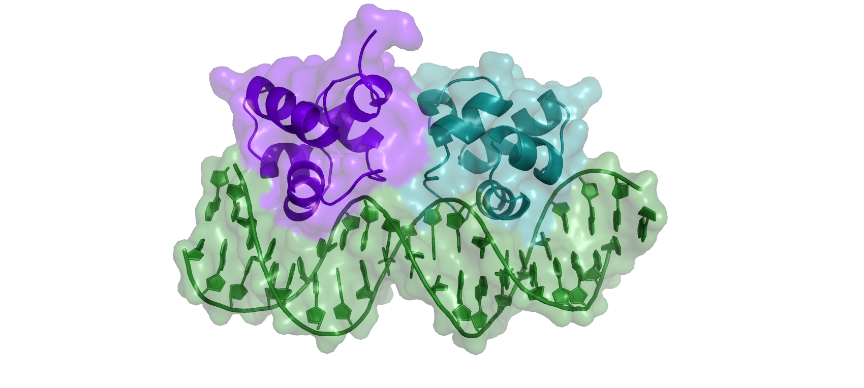
Figure 2: Cartoon representation of the X-ray structure (PDB id 3CRO) of the bacteriophage 434 Cro-OR1 complex.
Tutorial setup
The tutorial data is present as a zipped file in the following address https://surfdrive.surf.nl/public.php/dav/files/CuyiqNVryeN2wNz.
Extract the archive
You need to decompress the tutorial data archive. Move the archive to your working directory of choice and extract it.
1) Extract the archive in the current working directory:
tar /…/haddock-protein-dna-data.tgz
Extraction of the archive will present you with a new directory called 3CRO that contains a number of sub-directories arranged according to the part of this tutorial:
- part_1: Here, the data for the first protein-DNA docking run can be found and the results should be downloaded to.
- part_2: Here you will prepare the starting structures of the first docking run
- part_3: Here you will prepare the Ambiguous Interaction Restraints for the first docking run.
- part_4: Here you will prepare the ensemble of DNA starting structures for the second docking run.
- part_5: Here, the results of the second HADDOCK web server run will be downloaded to.
- tools: this directory contains a number of programs and scripts that will be used throughout the tutorial.
The part directories with arch in their name contain the pre-calculated data for every part.
These can be use as reference or in case you are short on time or access to the web server is limited or impossible.
The 3CRO directory itself contains the X-ray reference structure of the complex that we are going to dock (3CRO_complex.pdb).
Here, you will also find a setup script that will prepare the shell environment, so you can use all the tools available.
Change directory to the 3CRO directory and then set the environment by sourcing this file: setup.sh (.csh)
2) Set the shell environment by sourcing the setup script:
In case of a bash shell: >source setup.sh
In case of a C-shell: >source setup.csh
References
1) Dominguez, C. et al. (2003). HADDOCK: a protein-protein docking approach based on biochemical or biophysical information. JACS 125, 1731-1737
2) van Dijk, M. et al. (2006). Information-driven protein-DNA docking using HADDOCK: it is a matter of flexibility. Nucl. Acids. Res. 25, 3317-3325
3) van Dijk and Bonvin (2010) Pushing the limits of what is achievable in protein-DNA docking: benchmarking HADDOCK’s performance. Nucleic Acids Res 38, 5634-5647
4) Mondragón and Harrison (1991). The phage 434 Cro/OR1 complex at 2.5 A resolution. J Mol Biol 219, 321-334
Part I: Preparing the first HADDOCK2.4 docking run
The introduction of the HADDOCK web server in 2008 and the eNMR Grid-enabled web server shortly after, changed a lot in the docking community. HADDOCK 2.4 is now available for commercial use through https://wenmr.science.uu.nl/haddock2.4/ after registration. As the years progressed, new machine learning based modelling tools started to emerge, such as AlphaFold. Although machine-learning based methods eased modelling of a variety of protein-protein complexes, it cannot be used for protein-DNA or protein-RNA modelling. Therefore, HADDOCK remains a very convenient tool to be used for protein-DNA docking. The combination of automated setup procedures, vigorous checks of the input, best practice defaults, easy access to many of the powerful HADDOCK features and access to ample computer resources has made docking available to a wide audience.
Protein-DNA complexes are one of the more challenging systems to dock but also here the HADDOCK web server assists the user with several automated routines to setup the system correctly. This first part of the tutorial will introduce you to these features.
Using this part
With the protein and DNA starting structures available and the Ambiguous Interaction Restraints setup, you can start setting up your docking using the HADDOCK web server.
This part will introduce you to the use of the HADDOCK web server for the docking of protein-DNA systems. Although basic two-body protein-DNA docking can be performed using the HADDOCK Easy interface privileges, the use of custom Ambiguous Interaction Restraints requires the Expert privileges and the use of additional restraint types such as symmetry restraints, tweaking of the sampling parameters and multi-body docking requires the Guru privileges. Hence, for this tutorial you will require Guru access privileges. After registering to HADDOCK from here, you can request access elevation from here.
Protein-DNA docking using the HADDOCK web server
Apart from the default setup procedures and server input checks, the use of DNA requires two additional steps that are automatically performed by the server:
- The server will define the proper nucleic acid topology, parameter and linkage files for the partners indicated to be DNA. A ribose or deoxyribose patch will be applied depending on the choice of “Nucleic acid (DNA and/or RNA)” as input structure.
- An additional set of restraints will be generated to help maintain the helical structure of the DNA. These include sugar-pucker restraints, nucleotide base planarity restraints, sugar-phosphate backbone dihedral restraints and Watson-Crick hydrogen bond restraints between nucleotides that have been detected to be within pairing distance of one another.
In addition to these automatic setup procedures, there are a number of settings specific to protein-DNA docking that are worth considering:
- Flexibility: DNA often changes conformation globally in the vicinity of the interface of the protein. To allow such changes to occur, you need to define nearly the full DNA sequence as semi-flexible to allow the DNA to change conformation globally. Full flexibility is not recommended.
- Dielectric constant (epsilon): Is set to 78 on default for both it0 and it1.
- Advanced sampling parameters: the heating and cooling regime in the simulated annealing stages is optimized for protein systems but might be a bit too coarse for DNA systems. Reducing temperature, and the number and size of time steps will help in maintaining the helical structure of the DNA.
Preparing the Cro-OR1 docking run
Setup the Cro-OR1 multi-body docking run using HADDOCK 2.4 webserver.
Input files can be found in protein-DNA_basic directory.
Input data
Name –> Give your run a name. Molecules –> 3
Molecule 1 - input:
Molecule 2 - input:
Molecule 3 - input:
Click Next at the bottom of the page to proceed to “Input parameters” section.
This will upload the structures to the HADDOCK webserver where they will be processed and validated (checked for formatting errors).
The server makes use of Molprobity to check side-chain conformations, eventually swap them (e.g. for asparagines) and define the protonation state of histidine residues.
Input parameters
Molecule 3 (OR1) - parameters:
Click Next at the bottom of the page to proceed to “Docking parameters” section.
Docking parameters
Distance restraints:
Clustering parameters:
By default, the recommended cut-off value is 7.5 Å. However, because of the limited number of docking trials you performed with respect to the sampling requirements (due to flexibility and AIR restraints) the cut-off of 7.5 Å will not result in any clusters and hence no proper finalization of the docking run and it therefore increased to 20 Å. Under “normal” conditions (i.e. not this tutorial), the 7.5 Å cut-off is good value to use.
Symmetry restraints:
Energy and interaction parameters:
Advanced sampling parameters:
Click Submit at the bottom of the page to launch the docking.
Why is the full DNA structure defined as semi-flexible except for the terminal nucleotide pairs?
After your run has finished, you can download the output files of your run from the top of the page by clicking the hyperlink after “The complete run can be downloaded as a gzipped tar file”.
Extract the HADDOCK results from your first docking run (begin, data, structures, haddockparam.web, index.html, run.cns, and the four structures of the highest ranking two clusters) to the 3CRO/part_1 folder.
Finishing up
The first protein-DNA docking run between two ensembles of the monomeric Cro repressor and a DNA structural model for canonical OR1 is running on the HADDOCK server. The docking between the biomolecules is driven by your custom-built Ambiguous Interaction Restraint file and additional C2-symmetry restraints.
Depending on the available resources on the HADDOCK server your docking run will be finished within 2 to 3 hours. The pre-calculated results of this run are available in the part_1-arch directory, which will allow you to proceed with the tutorial.
In addition, a permanent link to the docking results of this tutorial is made available at the following link.
References
1) de Vries et al. (2010). The HADDOCK web server for data-driven biomolecular docking. Nat Protoc 5, 883-897
Part II: Preparing input structure files for the first HADDOCK run
Introduction
The quality of the HADDOCK generated structures depends very much on the quality of the input with respect to the structures of the individual molecules and the data used to dock them. Conformational deficiencies such as clashes, chain breaks and missing atoms may cause problems during the docking. This is also true for inconsistencies in the setup of the coordinates files in PDB format. Although the HADDOCK server performs a validation of the PDB structures you upload and can correct minor structural deficiencies, it is recommended to correct these beforehand. Furthermore, the conformation of the biomolecules in their unbound state may closely resemble their bound state but may also significantly differ. The degree of similarity between both states will determine, to a great extent, the efficiency of the flexible stages of the docking in reconstructing the complex.
Having control over the conformation of the input structures is unlikely for structures obtained via experimental means. Nevertheless, solving the structure by NMR of a protein in presence of its partner is a means of obtaining its structure in a bound conformation. Homology modelling approaches provide more control over the conformation but must be carefully checked for conformational deficiencies. For DNA, modelling approaches are often the only means of getting starting structures. Because of its regular build-up, DNA can be modelled in a much more controlled way than a protein. This benefit is used to efficiently deal with flexibility in protein-DNA systems.
Using this part
In this part we will introduce you to the various steps required to prepare PDB coordinate files for the Cro protein and the OR1 DNA structures. The procedure for the protein is no different than for protein-protein docking. You will be using an NMR-solved structure of the protein.
Modelling DNA is new to this tutorial and we will spend some more time discussing this part. You will be using the 3D-DART web server [1] for this purpose. This is certainly not the only way of generating DNA structural models and it is restricted to canonical double-stranded DNA only. It is nevertheless available as a convenient web server and provides detailed control over the conformation of the generated DNA models.
Running 3D-DART on a Docker Container
3D-DART server needs to be run on a Docker container to execute its function. Docker is a freely available software used to run applications reliably from one computing environment to another by the use of so-called containers (For more information: https://www.docker.com/resources/what-container/). By using Docker, you will be able to install and use the 3D-DART as a local server. Instructions on how to install 3D-DART are present on GitHub https://github.com/haddocking/3D-DART-server. It is also possible to run 3D-DART locally (https://github.com/haddocking/3D-DART), but nevertheless, it is not in the scope of this tutorial.
If you are following this tutorial on a Windows system, it is recommended to install WSL (Windows Subsystem for Linux) which allows for the execution of UNIX command line tools https://learn.microsoft.com/en-us/windows/wsl/install. Beware that Docker requires WSL 2 which you may need to update to run the application properly!
After you successfully manage to run 3D-DART container, the local server will be available from the url: http://127.0.0.1.
Preparing PDB coordinate files for protein-DNA systems
Obtaining starting structures and handling flexibility for DNA is one of the challenging aspects in protein-DNA systems. For various reasons, it is uncommon to obtain the structure of DNA in its unbound or bound conformation by experimental means. As such, modelling provides an appealing and often the only alternative to obtain starting structures.
Because of its assembly consisting of regular stacked nucleotides the DNA structure is an easy structure to model, at least for canonical double-stranded helixes. There are a number of considerations to make prior to modelling a DNA structure and using it in HADDOCK:
- The DNA sequence must be known. Such information can be acquired from DNA-foot printing experiments that are often conducted in the early stages of a biochemical characterization of the complex.
- The DNA conformational class: DNA is roughly categorized as belonging to A-, B- or Z-type conformational classes. Sub-categorization and mixed classes are nevertheless possible, especially for DNA in its bound conformation. Most ‘biologically active’ DNA is in a B-type conformation and this is a safe start point if not otherwise known.
- Does the DNA sequence contain unusual nucleosides? The HADDOCK topology definition currently includes the common nucleosides Adenosine, Cytidine, Guanosine, Thymidine and Uridine. Unusual nucleosides are not supported. The same is true for RNA.
- Does the conformation deviate from canonical double-stranded DNA? DNA conformational features such as gapped DNA, flipped-out bases, complex base pairing and loops are accepted by HADDOCK. They however might require an additional set of user-defined hydrogen bond restraints or unambiguous restraints to maintain the DNA conformation in addition to the default DNA restraints generated by the HADDOCK server. Different DNA modelling procedures might be required in these cases instead of, or in addition to 3D-DART.
Preparing PDB coordinate files for the OR1 operator
The structure of the OR1 operator is not known but its sequence has been determined by DNA foot printing techniques and thus we can model it. You will use the 3D-DART web server to generate a starting DNA model.
Generating the structure of OR1 operator
1) Generate a 3D structural model of the OR1 operator using the 3D-DART server. After you are sure that the container is running, navigate to http://127.0.0.1 to access the 3D-DART server.
Step 1:
name –> OR1
Sequence –> AAGTACAAACTTTCTTGTAT
Step 3:
Convert nucleic acid 1 letter to 3 letter notation –> Check
Submit the form once done. A download link to the results is usually returned in seconds.
2) Retrieve the 3D-DART server results
The web server will generate B-type DNA structures by default. The more advanced Nucleic Acid modelling options are not yet important.
Modifying the 3D-DART DNA model
The DNA model created by the 3D-DART server outputs a .pdb file that is not compatible with HADDOCK 2.4’s nucleic acid base notation (e.g. for Adenine residues HADDOCK 2.2 uses “ADE” while HADDOCK 2.4 uses “DA”). For more information regarding residue names, HADDOCK 2.4 library should be checked https://wenmr.science.uu.nl/haddock2.4/library.
To overcome this issue, .pdb file could be modified by the following command, which changes the residue names to their proper counterparts. Don’t forget to change the path to where the OR1_unbound.pdb file is located.
3) Change the nucleic acid residue names
Preparing PDB coordinate files for the Cro protein
The structure of the transcription factor Cro has been solved in its monomeric unbound conformation by NMR [2]. An ensemble of 20 structures has been deposited into the PDB with PDB id 1ZUG. The amino-acid side-chain and or main-chain conformations might differ between models in the ensemble. As such the ensemble represents a conformational space that might sample unbound and/or bound conformations.
The HADDOCK server accepts ensembles in the same way as they are deposited in the PDB (MODEL, ENDMDL separated). Such an ensemble is split into separated PDB files by the server that will start a docking run in which all single PDBs are used. Using these ensembles thus provides a means of including flexibility in the docking by implicit means.
An ensemble of 5 Cro proteins is available in the part_2, directory as 1ZUG_ensemble.pdb.
Finishing up
Both Cro protein and OR1 DNA structures are now ready for use with the HADDOCK web server.
References
1) van Dijk and Bonvin (2009). 3D-DART: a DNA structure modelling server. Nucleic Acids Res 37 (Web Server issue) pp. W235-239
2) Padmanabhan, S. et al. (1997) Three-dimensional solution structure and stability of phage 434 Cro protein. Biochemistry 36, 6424-6436
Part III: Understanding Ambiguous Interaction Restraints in Protein-DNA Docking
Introduction
The ability to use a wide range of information about a biomolecular complex as a direct means to drive the docking is one of the cornerstones of HADDOCKs versatility. Using both classical experimental data such as NMR distance restraints (e.g. NOE-based) as well as all biochemical and/or bioinformatics data you might have available about the complex, allows for a full integration of HADDOCK in an experimental structure determination workflow.
All data such as mutation data or interface prediction data, which cannot be expressed as a strict distance or angular restraint, are encoded as Ambiguous Interaction Restraints (AIRs). The network of restraints that is generated as such is a powerful way to reduce the search through conformational space and enrich the final solutions with relevant poses.
In this part we will introduce you to some of the more powerful methods for generating AIRs and make optimal use of the information content of the data you have at hand.
Using this part
The topics covered in this part assume that you are familiar with the concept of “Ambiguous Interaction Restraints” and their basic setup using active and passive residues (See Reference for more information).
In this part, you will use a custom-made plugin for the PyMOL molecular viewer to construct and visualise AIRs for the Cro-OR1 system. The plugin combines the ability to construct custom restraint sets for multi-body systems with the convenience of a visual appreciation of the resulting restraints network.
Note that AIRviewer is mainly useful when AIRs are generated by manually selecting residues in PyMOL. In most cases, it is more convenient and up to date to use the HADDOCK Generate Restraints web interface, the haddock-restraints command-line tool, or to simply specify active/passive residues directly in the Input parameters section of the HADDOCK web server.
Note that AIRviewer is not the only way to visualize the restraints network. You can also use haddock-restraints with the --pml flag. See the documentation for more details.
Constructing AIRs for protein-DNA systems
Generating Ambiguous Interaction Restraints for protein-DNA systems is accompanied with a number of challenges that require a different approach than for most of the common protein-protein systems:
- There are many multimeric protein-DNA systems. In these cases, the proteins often interact with more than one interaction site on the same DNA structure. The default way of generating restraints by linking all active/passive residue pairs over all partners thus creates too much ambiguity.
- A DNA nucleotide is a rather large ‘residue’ consisting of a base moiety and a sugar-phosphate backbone moiety. There is often specific information available that indicates that an amino acid only interacts with the base moiety for instance. AIR generation based on atom-subsets is thus preferable.
Reducing the ambiguity in multi-body restraints and using atom subsets is not possible using the default behaviour of the Easy HADDOCK web interface.
But the Expert and Guru privileges, the Multi-body interfaces will allow you to upload your own custom AIR restraint file.
Generating the restraint file using the PyMol plugin (AIRviewer.py), the online web server or by manually editing the files provides you with the flexibility you need to make AIRs work for your protein-DNA system.
Generating restraints for the CRO-OR1 complex
The CRO-OR1 test case is one of the model systems used by the scientific community to study transcription factors. There is a wide variety of biochemical data available for this complex, enough to be used in the docking.
Available data
A query of the information available in the scientific literature and several databases using structure and sequence data provides as with the following data on the CRO-OR1 system [1-4]:
- A domain search shows that this small α-helical protein uses a HTH (helix-turn-helix) motif for interaction with the DNA. HTH-motives predominantly interact with DNA major grooves.
- The helix α3 (residue 30-38) interacts specifically with the DNA while helix α2 (residue 19-26) interacts with the DNA backbone.
- There are a number of conserved residues in the HTH domain than might be important in DNA interaction. These are: K29, Q31, L35, S32
- The OR1 operator is pseudo-rotational symmetric.
- Ethylation interference experiments indicate that the nucleotides T4, A5, C14, T15, T22, A23, G31, T32, T33 are buried in the complex.
- Nucleotides: T4, A5, C6, A7, T13 C14, T15, T16, G17, T18, T22, A23, C24, A25, G31, T32, T33, T34, G35, T36 are conserved among many related sequences.
- Mutagenesis studies showed that at least L35 is involved in base-specific interaction to C14, T15 / T32, T33. Similarly, mutations of these nucleotides have been shown to abolish interaction. Also Q31 and S32 are proposed to be involved with specific interaction but there is no more info on the DNA side.
The data available for the OR1 operator provide a fairly detailed definition of the two binding interfaces that line up on the same face of the DNA. They are both major-groove binding sites that are rotationally symmetrical and separated by a short linker. Supported by the specific interaction between protein and DNA it becomes obvious that two protein monomers bind to the operator in a rotational symmetric fashion (i.e. C2-symetrical).
Because the monomers are identical and the operator has pseudo-rotation symmetry we can map the interaction from protein A to DNA B and from protein C to DNA B but we have no true interaction data between both proteins A and C.
Using the PyMol plugin to create the AIR file
You will now generate your custom AIR file using the PyMol AIR plugin (AIRviewer.py).
You will use the airsession.pdb file as a template.
This file contains all three input structures in one view to allow for an easy view of the whole system.
Setup PyMol by following these steps:
1) Open PyMol with the template file
cd 3CRO/part_3
load airsession.pdb
2) Setup PyMol to use the AIRviewer plugin
Click on Plugin»Plugin Manager on the top-right of the screen. A plugin menu will appear. Click on Install New Plugin, and Choose file.... Select AIRviewer.py, follow PyMol’s instructions.
Alternatively, on the PyMol Command line (1):
The sequence viewer can be used to select residues.
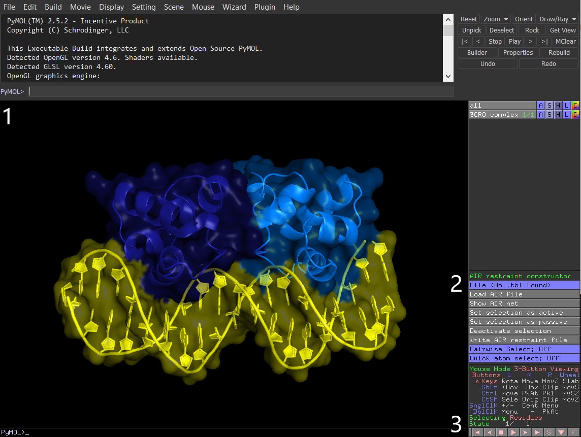
Figure 3: PyMol with activated AIRviewer plugin `AIRviewer.py`. 1) PyMol command line. 2) AIRviewer option buttons. 3) Bottom option bar with sequence viewer `S` activation button
The plugin is now activated and its functionality is available as a number of buttons on the right side panel (Figure 3.2). Let’s start constructing the restraint set for our system in 4 steps (3-6). All steps are performed in the same PyMol session:
Note that AIRviewer3 requires manual actvation every time new PyMOL window is open. To do so, go to Plugin Manager»Installed Plugins,
find AIRviewer3 in the list and click Load. Please note that it is mandatory to upload a complex to PyMOL before loading AIRviewer3.
If no molecules are open in PyMOL, AIRviewer3 loading will fail with the next error message:
ERROR: no chain ID and no segid ID defined. Need one of these object of type 'NoneType' has no len()
Unable to initialize plugin 'AIRviewer' (pmg_tk.startup.AIRviewer3)
3) Setup AIRs between conserved residues of helix 3 and nucleotide bases of OR1
4) Specific interaction between L35 and two nucleotides
5) (A)specific interactions between helix 3 and the DNA
6) Save the AIR restraints to file
You can view the restraint network by clicking the button ‘Show AIR net’. This will show the AIRs setup from A to B, C to B and vice versa (click the selections ‘Partner-A’, ‘Partner-B’ and ‘Partner-C’ to toggle them on and off). Selecting one or more residues and clicking the ‘Show AIR net’ button will show you the restraints specific to those residues.
Why are there more restraints from B to A than from A to B (same for C)?
Finishing up
You have now created a custom AIR file for the 3-body Cro-OR1 system using biochemical and bio-statistical data. You have reduced the overall ambiguity in the restraint set by defining only restraints between one protein monomer and one operator half side. Furthermore, you have setup restraints for the residues in the recognition helix of the protein to only target the bases of the nucleotides that are important in specific recognition and discarding the atoms belonging to the sugar-phosphate backbone. Finally, even specific amino acid to nucleotide-base restraints have been generated.
You are now ready for the next step: filling out the HADDOCK web server web form.
References
1) Harrison, S.C. et al. (1988). Recognition of DNA sequences by the repressor of bacteriophage 434. Biophys. Chem. 29 , 31-37
2) Koudelka, G.B. (1998) Recognition of DNA structure by 434 repressor. Nucleic Acids Res. 26, 669-675
3) Koudelka, G.B. et al. (1993). Differential recognition of OR1 and OR3 by bacteriophage 434 repressor and Cro. J. Biol. Chem. 268, 23812-23817
4) Wharton, R.P. et al. (1984). Substituting an alpha-helix switches the sequence-specific DNA interactions of a repressor. Cell. 38, 361-369
Part IV: Analysing the results of first docking run
Introduction
If you are not working on the pre-calculated data (accessible in the part_1-arch directory or using the following link), you have just retrieved the full server results archive of your first protein-DNA docking run.
That is exiting, but you are yet halfway!
You will have to analyse your first docking results with two objectives in mind:
- Do the first solutions look reasonable; are the restraints satisfied, to the solutions cluster into distinct clusters that are populated with a sufficient number of solutions.
- Did the DNA in the complexes changed conformation and is there a consensus in the distribution and extend of the conformational change.
The DNA analysis is the part unique to protein-DNA docking. The principles of this analysis and structure generation algorithm are described in the 3D-DART article [1]. In short, the protocol functions as follows:
- The conformation of the DNA in a selection of solutions is analysed and expressed in terms of 6 base pair and 6 base pair step parameters (Figure 4). These 6 parameters, each divided in 3 rotational and 3 translational parameters, uniquely describe the position of one base relative to its Watson-Crick partner and of two base pairs relative to each other from a local perspective.
- The base pair step parameters are transformed from a local reference frame to a global reference frame. A vector is calculated between neighbouring base pairs with respect to the global reference frame and thus represents a bend angle and direction. Added together these angles describe the global bend of the DNA helix.
- Statistics are calculated for all base pair and base pair step parameters and all global bend angles for all solutions in the selection.
- The consensus is used to model new 3D structural models. This process is in effect the opposite of the analysis procedure. Base pair and base pair step parameters are used to position bases building blocks in space. A sugar-phosphate backbone is added to connect the bases.
- Smart extrapolation of the global and local DNA conformational descriptors allows for sampling of conformations outside of the boundaries of the selection of solutions.
This protocol enables the generation of custom pre-bend and twisted DNA structural models. They preserve and build upon the essential motions introduced during the docking while removing any structural deformations.
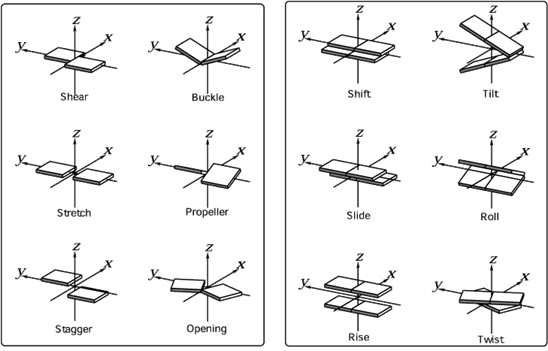
Figure 4: 6 base pair parameters (left) and six base pair-step parameters (right)
Analysing protein-DNA docking results
Analysing protein-DNA docking results consists of two parts; a general qualitative and quantitative inspection of the results as also performed for protein-protein docking and a DNA specific analysis.
First, the general analysis involves a visual inspection of the results. Have a look at the top-ranking solutions of each cluster. Do they look reasonable, how much do they differ from each other (e.a. do they cluster sufficiently). What types of contacts are present in the solutions, favourable ones such as hydrophobic contacts, electrostatic contacts, and hydrogen bonded interactions, or are they unfavourable such as electrostatic repulsions and buried charges. Do the numbers also correspond to your visual observations? With other words, do the various energies that are a part of the HADDOCK score rank the solutions in a sensible way?
At this stage it is also advisable to validate the solutions according to the information used to dock the structures. Pick a few active residues or perhaps NOEs and see if they are satisfied.
The DNA specific analysis focuses on the conformation of the DNA in the various solutions. Also, here a visual inspection is recommended. Does the DNA look reasonable with respect to its helical character, Watson-Crick pairing and backbone conformation? If the DNA changes conformation during interaction with the protein, we would like to know if this is consistent and if we can use it to generate new DNA structural models for use in the second docking run.
Because we use a protein-DNA test case for which the structure of the complex is known, we also would like to know to what extend the top-ranking solutions reassemble the reference structure. For this we use the CAPRI criteria [1] as quality assessment expressed as stars:
- “high quality” (3 CAPRI stars): Fnat > 0.5, l-RMSD or i-RMSD < 1.0 Å
- “medium quality” (2 CAPRI stars): Fnat > 0.3, l-RMSD < 5.0 Å or i-RMSD < 2.0 Å
- “acceptable quality” (1 CAPRI star): Fnat > 0.1, l-RMSD < 10.0 or i-RMSD < 4.0 Å
- “low quality” (none CAPRI star): Fnat < 0.1, l-RMSD > 10.0 or i-RMSD > 4.0 Å
Analysing the first Cro-OR1 docking solutions
Two scripts perform both the general analysis of the docking solutions as well as the more specific DNA analysis automatically.
Before running the analysis command, you should change the path to necessary scripts in the /tools/HaddockAnalysis/ folder.
To do that you can either manually open the Constants.py file with a ASCII editor to change the paths for profit, contact, and PDBXSEGCHAIN which are all in the /tools/HaddockAnalysis/ folder, or you can use the following command line tools separately by changing the path corresponding to where the /tools/HaddockAnalysis/ folder is located on your computer (Change the “∼” with your actual path to the folder.
If you have not done it yet, extract the HADDOCK results from your first docking run (begin, data, structures, haddockparam.web, index.html, run.cns, and the four structures of the highest ranking two clusters) to the 3CRO/part_1 folder before executing following commands.
1) General analysis of the protein-DNA docking solutions
Make sure you have enabled the right shell environment:
Navigate one directory below the tutorial data root (below 3CRO):
Execute the command:
analysis -r 3CRO/part_1/ -an complex
Wait till the process is finished (a few minutes).
The analysis program will generate a new directory in ‘part_1’ called ‘Analysis_3CRO_part_1’. The analysis.stat file contains a summary of various statistics of the best ranking solutions after rigid body docking (it0), semi-flexible refinement (it1 and water) and for every cluster.
Detailed statistics are provided for the 10 best solutions according to the HADDOCK score and according to i-RMSD to the reference in every stage. The same detailed statistics are listed for the 10 best solutions of every cluster according to the HADDOCK score (or less that 10 if the cluster is not so large). For all these cases the interface fitted structures are available in the directory and can be visualized with a molecular viewer.
2) Visualize the best solutions using PyMol
The docking solution and reference structure will be superimposed on each other.
Analysing the DNA structure in the best docking solution of the first run
The detailed DNA analysis and model building will be done with the 3D-DART server. The server accepts a .pdb file and outputs an analysis file that determines various properties of the DNA structure. To do this, the best model from the analysis must be chosen.
Observe the ranking of different structures and determine the best structure among them.
3) DNA analysis and custom DNA structure model generation combined using the 3D-DART server.
Be sure that your 3D-DART container is running and navigate to http://127.0.0.1 to access to 3D-DART server. Beware that you will upload to 3D-DART server the best structure that was determined by the analysis.
Step 1:
name –> OR1
Build from PDB structure file –> clust1_complex_x
4) Generate a new 3D structural model of the OR1 operator using the 3D-DART server.
Navigate to http://127.0.0.1 to access to 3D-DART server.
Step 1:
name –> OR1
Sequence –> AAGTACAAACTTTCTTGTAT
Step 2:
Define bend angle range (Global) –> (X-2)-(X+2)
Where X is the global bend angle computed by 3D-DART (e.g. if the bend angle is 25, it should be written as 23-27).
5) Join the .pdb files in a single pdb ensemble file and change residue names.
To join the various pdb files previously generated, use with the following set of commands.
cd 3CRO/part_4/
./joinpdb.sh -o OR1_ensemble.pdb OR1*_fixed.pdb
Then, once again, use the sed command to modify base names to fit current naming:
sed -i -e “s/ADE/ DA/g” -e “s/CYT/ DC/g” -e “s/GUA/ DG/g” -e “s/THY/ DT/g” OR1_ensemble.pdb
Finishing up
Upon analysis of the docking results of the first docking run, you have generated a new ensemble of custom DNA structural models. These pre-bend and twisted models build upon the conformational changes introduced in the first docking run. The ensemble preserves the essential motions and removes any structural distortions. You are now ready to use it as input for a second docking run.
It is important to note that the quality of the ensemble of custom DNA structural models you generated directly depends on the docking solutions of the first run. Aspects such as: the conformational space sampled (number of docking trials), the convergence of the solutions in the clusters and the number of solutions in the top-ranking cluster all influence the acquired statistics in the DNA analysis stage and thus the quality of the generated models ensemble.
References
1) van Dijk and Bonvin (2009). 3D-DART: a DNA structure modelling server. Nucleic Acids Res 37 (Web Server issue) pp. W235-239
Preparing the second HADDOCK run
Introduction
The second and last protein-DNA HADDOCK run is a continuation of the first. It is performed in almost the same way, with the only difference being the use of custom DNA structural models ensembles we just created.
Preparing the second Cro-OR1 docking run
Input data
Name –> Give your run a name
Molecules –> 3
Molecule 1 - input:
Molecule 2 - input:
Molecule 3 - input:
Click Next at the bottom of the page to proceed to Input parameters section.
This will upload the structures to the HADDOCK webserver where they will be processed and validated (checked for formatting errors).
The server makes use of Molprobity to check side-chain conformations, eventually swap them (e.g. for asparagines) and define the protonation state of histidine residues.
Input parameters
Molecule 3 - parameters:
Click Next at the bottom of the page to proceed to Docking parameters section.
Docking parameters
Distance restraints:
Clustering parameters:
Clustering method –> RMSD
RMSD cutoff for clustering –> 20Å
Minimum cluster size –> 4
Symmetry restraints:
Energy and interaction parameters:
Advanced sampling parameters:
Once all the webserver forms have been filled out as described above you can click on Submit button at the bottom of the page and select “No” for the “Do you want to tag this job as COVID-19 related research?” selection.
The web form will first be validated.
Once done, it will be added to the job queue and start running when resources are available.
You will be notified by email once your job is added to the queue and afterwards on the continuation of your job.
After your run has finished, you can download the output files of your run from the top of the page by clicking the hyperlink after “The complete run can be downloaded as a gzipped tar file”.
Extract the HADDOCK results from your first docking run (begin, data, structures, haddockparam.web, index.html, run.cns, and the four structures of the highest ranking two clusters) to the 3CRO/part_5 folder.
Pre-calculated dockign result are accessible for you to run the analysis on, if time runs short.
It is available at the following adress an also present in the 3CRO/part_5-arch folder.
Once your second docking run is downloaded locally on your computer, you may use the same general analysis procedure as described in part IV to visualize and quantify the progress with respect to the first docking run.
Analyzing the second Cro-OR1 docking solutions
1) General analysis of the protein-DNA docking solutions
Extract the HADDOCK results (begin, data, structures, haddockparam.web, index.html, run.cns, and the four structures of the highest ranking two clusters) to the 3CRO/part_5 folder before executing following commands.
Make sure you have enabled the right shell environment:
Navigate one directory below the tutorial data root (below 3CRO):
Execute the analysis command on the appropriate directory:
analysis -r 3CRO/part_5/ -an complex
Wait till the process is finished (it may take few minutes).
Observe the ranking of different structures and determine the best structure among them.
2) Visualize the best solutions using PyMol
Compare the best structure of the first analysis, second analysis, and reference structure visually in PyMol.
The docking solution and reference structure will be superimposed on each other.
Congratulations!
You have made it to the end of this advanced protein-DNA docking tutorial. We hope it has been illustrative and may help you get started with your own docking projects.
Happy Haddocking!