

Integrative modelling of the apo RNA-Polymerase-III complex from MS cross-linking and cryo-EM data
This tutorial consists of the following sections:
- Introduction
- Setup/Requirements
- HADDOCK general concepts
- The information at hand
- Inspecting the AlphaFold models
- Using DISVIS to visualize the interaction space and filter false positive restraints
- Strategy 1): Modelling the complex (core + C82 + C34wHTH1 + C34wHTH2 + C31peptides) by docking with cross-links
- Strategy 2): Modelling the complex by docking with cross-links only, using as starting conformations the models fitted into the cryo-EM map
- Introduction to PowerFit
- Fitting PolIII-core and C82+C34wHTH3 into the 9Å cryo-EM map
- Refining the fit in Chimera
- Refining the interface of the cryo-EM fitted models with HADDOCK
- Checking the agreement of the refined cryo-EM fitted models with the cross-links
- Setting up the full docking run using the cryo-EM fitted and refined core and C82 domains
- First analysis of the docking results
- Visualisation of docked models
- Satisfaction of cross-link restraints
- Fitting the docking models into low resolution cryo-EM maps
- Conclusions
- Alternative runs
- Congratulations!
Introduction
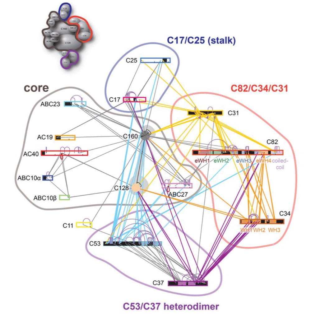
This tutorial will demonstrate the use of our DISVIS, POWERFIT and HADDOCK web servers for predicting the structure of a large biomolecular assembly from MS cross-linking data and low resolution cryo-EM data. The case we will be investigating is the apo form of the Saccharomyces cerevisiae RNA Polymerase-III (Pol III). Pol III is a 17-subunit enzyme that transcribes tRNA genes. Its architecture can be subdivided into a core, stalk, heterodimer of C53 and C37, and heterotrimer of C82, C34, and C31 subunits.
During this tutorial, we pretend that the structure of the Pol III core (14 subunits) is known. Therefore, we will focus on modeling the positioning of the C82/C34/C31 heterotrimer subunits relatively to the others (which we will treat as the core of Pol III). The structure of Pol III core is quite well characterized, with multiple cryo-EM structures of Pol III published.
We will be making use of i) our DISVIS server to analyse the cross-links and detect possible false positives and ii) of the new HADDOCK2.4 webserver to setup docking runs, using the coarse-graining option to speed up the calculations (especially needed due to the large size of the system). As an alternative strategy, we will use our PowerFit server to fit the largest components of the complex into the 9Å cryo-EM map and then use those as a starting point for the modelling of the remaining components.
- R.V. Honorato, M.E. Trellet, B. Jiménez-García1, J.J. Schaarschmidt, M. Giulini, V. Reys, P.I. Koukos, J.P.G.L.M. Rodrigues, E. Karaca, G.C.P. van Zundert, J. Roel-Touris, C.W. van Noort, Z. Jandová, A.S.J. Melquiond and A.M.J.J. Bonvin. The HADDOCK2.4 web server: A leap forward in integrative modelling of biomolecular complexes. Nature Prot., Advanced Online Publication DOI: 10.1038/s41596-024-01011-0 (2024).
Throughout the tutorial, colored text will be used to refer to questions or instructions, and/or PyMOL commands.
This is a question prompt: try answering it! This an instruction prompt: follow it! This is a PyMOL prompt: write this in the PyMOL command line prompt! This is a Linux prompt: insert the commands in the terminal!
Setup/Requirements
In order to follow this tutorial you will need a web browser, a text editor, PyMOL and Chimera (both freely available for most operating systems) to visualize the input and output data. We used our pdb-tools to pre-process PDB files for HADDOCK, renumbering the core domains to avoid overlap in their residue numbering. Ready to dock models are provided as part of the material for this tutorial. The required data to run this tutorial should be downloaded from here. Once downloaded, make sure to unpack/unzip the archive (for Windows system you can install the 7-zip software if needed to unpack tar archives).
Also, if not provided with special workshop credentials to use the HADDOCK portal, make sure to register in order to be able to submit jobs. Use for this the following registration page: https://wenmr.science.uu.nl/auth/register/haddock.
HADDOCK general concepts
HADDOCK (see https://www.bonvinlab.org/software/haddock2.4) is a collection of python scripts derived from ARIA (https://aria.pasteur.fr) that harness the power of CNS (Crystallography and NMR System, http://cns-online.org/v1.3/) for structure calculation of molecular complexes. What distinguishes HADDOCK from other docking software is its ability, inherited from CNS, to incorporate experimental data as restraints and use these to guide the docking process alongside traditional energetics and shape complementarity. Moreover, the intimate coupling with CNS endows HADDOCK with the ability to actually produce models of sufficient quality to be archived in the Protein Data Bank.
A central aspect to HADDOCK is the definition of Ambiguous Interaction Restraints or AIRs. These allow the translation of raw data such as NMR chemical shift perturbation or mutagenesis experiments into distance restraints that are incorporated in the energy function used in the calculations. AIRs are defined through a list of residues that fall under two categories: active and passive. Generally, active residues are those of central importance for the interaction, such as residues whose knockouts abolish the interaction or those where the chemical shift perturbation is higher. Throughout the simulation, these active residues are restrained to be part of the interface, if possible, otherwise incurring in a scoring penalty. Passive residues are those that contribute to the interaction, but are of less importance. If such a residue does not belong in the interface there is no scoring penalty. Hence, a careful selection of the active and passive residues is critical for the success of the docking.
The docking protocol of HADDOCK was designed so that the molecules experience varying degrees of flexibility and different chemical environments, and it can be divided in three different stages, each with a defined goal and characteristics:
-
1. Randomization of orientations and rigid-body minimization (it0)
In this initial stage, the interacting partners are treated as rigid bodies, meaning that all geometrical parameters such as bonds lengths, bond angles, and dihedral angles are frozen. The partners are separated in space and rotated randomly about their centers of mass. This is followed by a rigid body energy minimization step, where the partners are allowed to rotate and translate to optimize the interaction. The role of AIRs in this stage is of particular importance. Since they are included in the energy function being minimized, the resulting complexes will be biased towards them. For example, defining a very strict set of AIRs leads to a very narrow sampling of the conformational space, meaning that the generated poses will be very similar. Conversely, very sparse restraints (e.g. the entire surface of a partner) will result in very different solutions, displaying greater variability in the region of binding.See animation of rigid-body minimization (it0):
-
2. Semi-flexible simulated annealing in torsion angle space (it1)
The second stage of the docking protocol introduces flexibility to the interacting partners through a three-step molecular dynamics-based refinement in order to optimize the interface packing. It is worth noting that flexibility in torsion angle space means that bond lengths and angles are still frozen. The interacting partners are first kept rigid and only their orientations are optimized. Flexibility is then introduced in the interface, which is automatically defined based on an analysis of intermolecular contacts within a 5Å cut-off. This allows different binding poses coming from it0 to have different flexible regions defined. Residues belonging to this interface region are then allowed to move their side-chains in a second refinement step. Finally, both backbone and side-chains of the flexible interface are granted freedom. The AIRs again play an important role at this stage since they might drive conformational changes.See animation of semi-flexible simulated annealing (it1):
-
3. Refinement in Cartesian space with explicit solvent (water)
The final stage of the docking protocol allows to immerse the complex in a solvent shell to improve the energetics of the interaction. HADDOCK currently supports water (TIP3P model) and DMSO environments. The latter can be used as a membrane mimic. In this short explicit solvent refinement the models are subjected to a short molecular dynamics simulation at 300K, with position restraints on the non-interface heavy atoms. These restraints are later relaxed to allow all side chains to be optimized. In the 2.4 version of HADDOCK, the explicit solvent refinement is replaced by default by a simple energy minimisation as benchmarking has shown solvent refinement does not add much to the quality of the models. This allows to save time.See animation of refinement in explicit solvent (water):
The performance of this protocol depends on the number of models generated at each step. Few models are less probable to capture the correct binding pose, while an exaggerated number will become computationally unreasonable. The standard HADDOCK protocol generates 1000 models in the rigid body minimization stage, and then refines the best 200 (ranked based on the HADDOCK score) in both it1 and water. Note, however, that while 1000 models are generated by default in it0, they are the result of five minimization trials and for each of these the 180 degrees symmetrical solution is also sampled. Thus, the 1000 models written to disk are effectively the sampling results of the 10.000 docking poses.
The final models are automatically clustered based on a specific similarity measure - either the positional interface ligand RMSD (iL-RMSD) that captures conformational changes about the interface by fitting on the interface of the receptor (the first molecule) and calculating the RMSDs on the interface of the smaller partner, or the fraction of common contacts (current default) that measures the similarity of the intermolecular contacts. For RMSD clustering, the interface used in the calculation is automatically defined based on an analysis of all contacts made in all models.
The new 2.4 version of HADDOCK also allows to coarse grain the system, which effectively reduces the number of particles and speeds up the computations. We are using for this the MARTINI2.2 force field, which is based on a four-to-one mapping of atoms on coarse-grained beads.
The information at hand
Let us first inspect the available data, namely the various structures (or AlphaFold models) as well as
the information from MS we have at hand to guide the docking. After unpacking the archive provided for this tutorial (see Setup above),
you should see a directory called RNA-Pol-III with the following subdirectories in it:
-
cryo-EM: This directory contains a 9Å cryo-EM map of the RNA Pol III (PolIII_9A.mrc).
-
disvis: This directory contains text files called
xlinks-all-X-Y.disvisdescribing the cross-links between the various domains (X and Y). These files are in the format required to run DISVIS. The directory also containts the results of DISVIS analysis of the various domain pairs as directories nameddisvis-results-X-Y - docking: This directory contains json files containing all the parameters and input data for HADDOCK. Those are reference files of the docking setup and allow to repeat the modelling using the
Submit Fileoption of the HADDOCK2.4 web server:strategy1-RNA-PolIII-core-C82-C34-C31pept.json: Docking following Strategy 1 as described in this tutorialstrategy2-RNA-PolIII-core-C82-EMfit-C34-C31pept.json: Docking following Strategy 2 as described in this tutorial
- input-pdbs: This directory contains the HADDOCK-ready input PDB files for the various domains
A_PolIII-5fja-core.pdb: The core region of Pol III with non-overlapping residue numbering (chain A)B_C82-alphafold-trimmed.pdb: The AlphaFold model of C82 excluding the disordered long loops (chain B)BE_C82-C34-wHTH3-alphafold-trimmed.pdb: The AlphaFold-multimer model of C82 and the third helix-turn-helix domain of C34 excluding the disordered long loops (chains B + E)C_C34_wHTH1-alphafold.pdb: The AlphaFold model of the first helix-turn-helix domain of C34 (chain C)D_C34_wHTH2-alphafold.pdb: The AlphaFold model of the second helix-turn-helix domain of C34 (chain D)F_C31_alphafold.pdb: The AlphaFold model of C31 - an unreliable model (chain F)F_C31_alphafold-K91-peptide.pdb: The peptide containing Lysine 91 from C31 AlphaFold model (chain F)G_C31_alphafold-K111-peptide.pdb: The peptide containing Lysine 111 from C31 AlphaFold model (chain G)
- restraints:
xlinks-all-core-C82-C34-C31-K91-K111.tbl: This file contains all cross-links between the core, C82, C34 domains and two peptides containing Lys 91 and Lys 111 from the C31 domain (chains F and G, respectively)C31-C34-connectivities.tbl: Connectivity restraints between the C34 domains and between the C31 peptidesrestraints-combined.tbl: The combination of those two files
- AF-multimer:
C82-C34-wo-template: AF-multimer run results for predicting C82-C34 binding.fasta-seqs: Fasta sequences for the mobile monomers that can be used for further AF2 modeling.
From MS, we have experimentally determined cross-links between the various domains. We have only kept here the inter-domain cross-links relevant for this tutorial.
The cross-links are taken from (Ferber et al. 2016. These are the files present in the disvis directory. As an example here
are the cross-links identified between the C82 (chain B here) and C34 (chain C):
B 520 CB C 135 CB 0.0 30.0
B 520 CB C 138 CB 0.0 30.0
B 520 CB C 141 CB 0.0 30.0
This is the format used by DisVis to represent the cross-links. Each cross-link definition consists of eight fields:
- chainID of the 1st molecule
- residue number
- atom name
- chainID of the 2nd molecule
- residue number
- atom name
- lower distance limit
- upper distance limit
Inspecting the AlphaFold models
For C82, C34, and C31, we will make use of the AlphaFold models. Before downloading those models from the AlphaFold Database and use them blindly for modelling, it is crucial to first carefully assess their quality. For docking purposes the disordered regions should be removed as those will only lead to problems during the modelling.
How should we interpret AlphaFold’s predictions? What are the predicted LDDT (pLDDT), PAE, iptm?
Tip: Try to find information about the prediction confidence at https://alphafold.ebi.ac.uk/faq. A nice summary can also be found here.
Let’s now take a look at the models for the three monomers that we want to dock (C82, C34, and C31).
C82 AlphaFold model
The C82 AlphaFold model can be accessed here.
Inspect the 3D model and in particular the color-coding which indicates the model confidence.
Also consider the Predicted aligned error displayed as a matrix.
Can you identify the poorly predicted regions?
See the AlhpaFold model and PAE plot
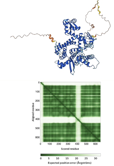
A trimmed model of C82 has been provided with the data for this tutorial. Inspect it in PyMol or your favourite 3D structure viewer.
What are the differences with the model from the AlphaFold database?
C34 AlphaFold model
The C34 AlphaFold model can be accessed here.
Inspect the 3D model and in particular the color-coding which indicates the model confidence.
Also consider the Predicted aligned error displayed as a matrix.
Can you identify the poorly predicted regions?
See the AlhpaFold model and PAE plot
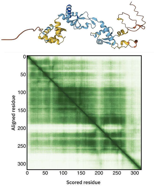
C34 consists of three winged-helix-turn-helix (wHTH) domains.
Can you identify them in the model?
Tip: In the AlphaFold page you can select a block in the PAE matrix that will automatically be highlighted in the model.
How well defined are the three wHTH domains?
Tip: To assess how well defined the relative positions of the domains are consider the off-diagonal blocks of the PAE matrix connecting them.
Since we do have a number of cross-links between wHTH1 and wHTH2, let’s check if the AlphaFold model satisfies those. For this we will inspect in PyMol the provided trimmed model of C34.
Start PyMOL and load the trimmed C82 model (C_C34-alphafold-trimmed.pdb):
File menu -> Open -> select C_C34-alphafold-trimmed.pdb
Note: If using the command line, simply type:
pymol C_C34-alphafold-trimmed.pdb
Let’s now check if this model actually fit the cross-links identified between the first two wHTH domains.
In the PyMOL command window type:
This will draw lines between the connected atoms and display the corresponding Euclidian distance. Objects are created in the left panel with their name corresponding to the cross-link and its associated maximum distance.
Inspect the various cross-link distances.
Is the model satisfying the cross-link restraints?
If not, which ones are not satistified?
Note that the reported distances are Euclidian distances. In reality, the cross-linker will have to follow the surface of the molecule which might results in a longer effective distance. A proper comparison would require calculating the surface distance instead. Such an analysis can be done with the XWalk or jwalk software.
C82-C34 AlphaFold-multimer model
We have generated this model using the Colab version of Alphafold. The results are provided in the data you downloaded in the AF2-multimer/C82-C34-wo-template directory. You can inspect the pdb models together with the png files, which contains the plDDT and PAE analysis calculated per model. For coloring the pdb files according to the plDDT scores, you can use the following PyMOL command:
File menu -> Open -> select C82C34_873a4_unrelaxed_rank_1_model_1.pdb
In the PyMOL command window type:
spectrum b, tv_red yellow cyan blue, minimum=30, maximum=100
Consider the Predicted aligned error displayed as a matrix.
Can you identify the poorly predicted regions? Focus here on the different domains.
See the AlhpaFold-multimer PAE plot
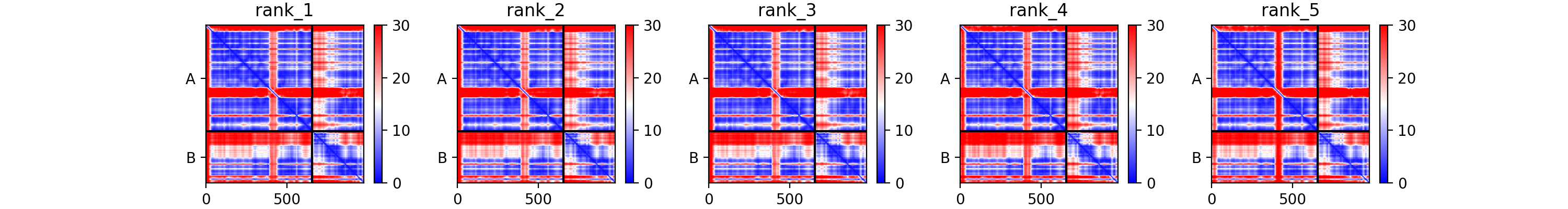
Which one of the three C34 wHTH domain orientation is best defined with respect to C82?
See answer
From an analysis of the diagonal blocks we can identify the three wHTH domains, whose stucture is well predicted. When considering the off-diagonal blocks, the last domain of C34, wHTH3, seems to be the best defined with respect to C82. We will make use of this in our modelling strategy 2 in this tutorial. Since the orientation of the other domains are not well defined with respect with C82, we will treat them as separate entities during our modelling.
C31 AlphaFold model
The C31 AlphaFold model can be accessed here.
Inspect the 3D model and in particular the color-coding which indicates the model confidence.
Also consider the Predicted aligned error displayed as a matrix.
How much trust to you have in this model?
See the AlhpaFold model and PAE plot
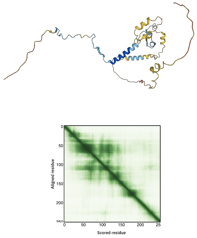
It should be rather evident that the prediction confidence for C31 is low. As such it does not make sense to use it as is during the modelling. But since there are a number of detected cross-links for this domain, in particular with the core and the C82 domains, we could consider including peptide fragments around the cross-linked lysines in the modelling. This will be illustrated below in Strategy 1.
Using DISVIS to visualize the interaction space and filter false positive restraints
Introduction to DISVIS
DisVis is a software developed in our lab to visualise and quantify the information content of distance restraints between macromolecular complexes. It is open-source and available for download from our Github repository. To facilitate its use, we have developed a web portal for it.
DisVis performs a full and systematic 6 dimensional search of the three translational and rotational degrees of freedom to determine the number of complexes consistent with the restraints. It outputs information about the inconsistent/violated restraints and a density map that represents the center-of-mass position of the scanned chain consistent with a given number of restraints at every position in space.
DisVis requires three input files: atomistic structures of the biomolecules to be analysed and a text file containing the list of distance restraints between the two molecules . This is also the minimal required input for the web server to setup a run.
DisVis and its webserver are described in:
-
G.C.P. van Zundert, M. Trellet, J. Schaarschmidt, Z. Kurkcuoglu, M. David, M. Verlato, A. Rosato and A.M.J.J. Bonvin. The DisVis and PowerFit web servers: Explorative and Integrative Modeling of Biomolecular Complexes.. J. Mol. Biol.. 429(3), 399-407 (2016).
-
G.C.P van Zundert and A.M.J.J. Bonvin. DisVis: Quantifying and visualizing accessible interaction space of distance-restrained biomolecular complexes. Bioinformatics 31, 3222-3224 (2015).
Analysing the Pol III domain-domain interactions with DISVIS
Before modelling Pol III, we will first run DisVis using the cross-links for the various pairs of domains to both assess the information content of the cross-links and detect possible false positives. For the latter, please note that DisVis does not account for conformational changes. As such, a cross-link flagged as possible false positive might also simply reflect a conformational change occuring upon binding.
We have cross-links available for 9 pairs of domains (see the disvis directory from the downloaded data). As an illustration of running DisVis, we will here
setup the analysis for the Pol III C82 (chain B) - C34 (chain C) pair.
To run DisVis, go to
https://wenmr.science.uu.nl/disvis
On this page, you will find the most relevant information about the server, as well as the links to the local and grid versions of the portal’s submission page.
Step1: Register to the server (if needed) or login
Register for getting access to the web server (or use the credentials provided in case of a workshop).
You can click on the “Register” menu from any DisVis page and fill the required information. Registration is not automatic but is usually processed within 12h, so be patient.
If you already have credential, simply login in the upper right corner of the disvis input form
Step2: Define the input files and parameters and submit
Click on the “Submit” menu to access the input form.
From the input-pdbs directory select:
Fixed chain → B_C82-alphafold-trimmed.pdb Scanning chain → C_C34-alphafold-trimmed.pdb
From the disvis directory select:
Restraints file → xlinks-C82-C34.disvis
Once the fields have been filled in, you can submit your job to our server by clicking on “Submit” at the bottom of the page.
If the input fields have been correctly filled you should be redirected to a status page displaying a message indicating that your run has been successfully submitted. While performing the search, the DisVis web server will update you on the progress of the job by reloading the status page every 30 seconds. The runtime of this example case is less than 5 minutes on our local CPU and grid GPU servers. However the load of the server as well as pre- and post-processing steps might substantially increase the waiting time.
If you want to learn more about the meaning of the various parameters, you can go to:
https://wenmr.science.uu.nl/disvis
Then click on the “Help/Manual” menu.
The rotational sampling interval option is in
degrees and defines how tightly the three rotational degrees of freedom will be
sampled. Voxel spacing is the size of the grid’s voxels that will be cross-correlated during the 3D translational search.
Lower values of both parameters will cause DisVis to perform a finer search, at the
expense of increased computational time. The default values are 15° and 2.0Å for a quick scanning and 9.72° and 1.0Å
for a more thorough scanning.
For the sake of time, in this tutorial we will keep the sampling interval as the quick scanning settings (15.00° and 2.0Å).
The number of processors used for the calculation is fixed to 8 processors on the web server side.
This number can of course be changed when using the local version of DisVis.
Analysing the results
Once your job has completed, and provided that you did not close the status page, you will be automatically redirected to the results page (you will also receive an email notification).
If you don’t want to wait for your run to complete, you can access the pre-calculated results in the data folder you downloaded for this tutorial.
Look for the disvis/disvis-results-C82-C34 directly and open in your web browser the results.html file present in that directory.
The results page presents a summary split into several sections:
Status: In this section you will find a link from which you can download the output data as well as some information about how to cite the use of the portal.Accessible Interaction Space: Here, images of the fixed chain together with the accessible interaction space (in a density map representation) are displayed. Different views of the molecular scene can be chosen by clicking on the right or left part of the image frame. Each view shows the accessible space consistent with the selected number of restraints (using the slider below the picture).Accessible Complexes: Summary of the statistics for the number of complexes consistent with at least N number of restraints. The statistics are displayed for the N levels, N being the total number of restraints provided in the restraints file (herexlinks-C82-C34.disvis)z-Score: For each restraint provided as input, a z-Score is calculated, indicating the likelihood that a restraint is a false positive. The higher the score, the more likely it is that a restraint is a false positive. Putative false positive restraints are only highlighted if no single solution was found to be consistent with the total number of restraints provided. If DisVis finds complexes consistent with all restraints, the z-Scores are still displayed, but in this case they should be ignored.Violations: The table in this sections shows how often a specific restraint is violated for all models consistent with a given number of restraints. The higher the violation fraction of a specific restraint, the more likely it is to be a false positive. Column 1 shows the number of restraints (N) considered, while each following column indicates the violation fractions of a specific restraint for complexes consistent with at least N restraints. Each row thus represents the fraction of all complexes consistent with at least N restraints that violated a particular restraint. As for the z-Scores, if solutions are found that are consistent with all restraints provided, this table should be ignored.
As mentioned above, the two last sections feature a table that highlights putative false positive restraints based on their z-Score and their violation frequency for a specific number of restraints. We will naturally look for the crosslinks with the highest number of violations. The DisVis web server preformats the results in a way that false positive restraints are highlighted and can be spotted at a glance.
In our case, you should observe that DisVis found solutions consistent with all 3 restraints submitted for C82-C34 interaction.
When DisVis fails to identify complexes consistent with all provided restraints during quick scanning, it is advisable to rerun with the complete scanning parameters before removing all restraints (or removing only the most violated ones and rerunning with complete scanning). It is possible that a more thourough sampling of the interaction space will yield complexes consistent with all restraints or at least reduce the list of putative false positive restraints.
DisVis output files
It is difficult to appreciate the accessible interaction space between the two partners with static images only. Therefore you should download the results archive to your computer (which is available at the top of your results page). You will find in the archive the following files:
accessible_complexes.out: A text file containing the number of complexes consistent with a number of restraints.accessible_interaction_space.mrc: A density file in MRC format. The density represents the space where the center of mass of the scanning chain can be placed while satisfying the consistent restraints.violations.out: A text file showing how often a specific restraint is violated for each number of consistent restraints.z-score.out: A text file giving the z-score for each restraint. The higher the score, the more likely the restraint is a false positive.run_parameters.json: A text file containing the parameters of your run.
Note: Results for the different pair combinations are available from the tutorial data directory in the disvis directory as disvis-results-X-Y.
Let us now inspect the solutions and visualise the interaction space in Chimera:
Open the fixed_chain.pdb file and the accessible_interaction_space.mrc density map in Chimera.
UCSF Chimera Menu → File → Open… → Select the file
Or from the Linux command line:
chimera fixed_chain.pdb accessible_interaction_space.mrc
The values of the accessible_interaction_space.mrc slider bar correspond to the number of satisfied restraints (N).
In this way, you can selectively visualise regions where complexes have been found to be consistent with a given number of
restraints. Try to change the level in the “Volume Viewer” to see how the addition of restraints reduces
the accessible interaction space.
Note: The interaction space displayed corresponds to the region of space where the center of mass of the scanning molecule can be placed while satisfying a given number of restraints
Remember that the displayed interaction space is the region where the center of mass of the second molecule can be put while satistying the distance restraints, contacting and not clashing with the first molecule.
Converting DISVIS restraints into HADDOCK restraints
In principle you should repeat the DisVis analysis for all pairs to detect possible false positives. For the provided data, however, all cross-links can be satisfied simultaneously, i.e. DISVIS does not identify false positives. Before setting up the docking, we need to generate the distance restraint file for the cross-links in a format suitable for HADDOCK. HADDOCK uses CNS as its computational engine. A description of the format for the various restraint types supported by HADDOCK can be found in our Nature Protocols paper, Box 4.
Distance restraints are defined as:
assi (selection1) (selection2) distance, lower-bound correction, upper-bound correction
The lower limit for the distance is calculated as: distance minus lower-bound correction and the upper limit as: distance plus upper-bound correction
The syntax for the selections can combine information about chainID - segid keyword -, residue number - resid
keyword -, atom name - name keyword.
Other keywords can be used in various combinations of OR and AND statements. Please refer for that to the online CNS manual.
As an example, a distance restraint between the CB carbons of residues 10 and 200 in chains A and B with an allowed distance range between 10 and 20Å can be defined as:
assi (segid A and resid 10 and name CB) (segid B and resid 200 and name CB) 20.0 10.0 0.0
Under Linux (or OSX), this file can be generated automatically from the xlinks-all-inter-disvis-filtered.disvis
file provided with the data for this tutorial by giving the following command (one line) in a terminal window:
The correspondong pre-generated CNS/HADDOCK formatted restraints files are provided in the restraints directory as:
xlinks-all-core-C82-C34.tblxlinks-all-core-C82-C34-C31-K91-K111.tbl(for use when including peptide fragments of C31)
Inspect the xlinks-all-core-C82-C34.tbl file (open it as a text file)
See solution:
Additional atoms are included in the distance restraints definitions: `BB`. These correspond to the backbone beads in the MARTINI representation.
In the restraints directory provided, there are additional restraint file provided, e.g.: C31-C34-connectivities.tbl.
Inspect its content.
What are those restraints for?
See solution:
C34 consists of three winged-helix-turn-helix domains which could be docked separately in principle. These are connected by flexible linkers. The defined restraints impose upper limits to the distance between the C- and N-terminal domains of the the domains. The upper limit was estimated as the number of missing segments/residues * 4.5Å (a typical distance observed in diffraction data for amyloid fibrils, representing a CA-CA distance in an extended conformation). The same applies to C31 for which only two peptide fragments will be used to be able to make use of the cross-link restraints.
Note: You should notice that the restraints are duplicated (actually 4 times). This is a way to tell HADDOCK to give more weight to those restraints.
Strategy 1): Modelling the complex (core + C82 + C34wHTH1 + C34wHTH2 + C31peptides) by docking with cross-links
We will use the core domain of RNA-PolIII together with the trimmed AlphaFold models of C82 and C34, and two peptides extracted from the C31 model.
For this we will set up a five-body docking using the PolIII-core, C82 and C34 and two peptides from C31:
- 1st molecule - chainA: PolIII-core
- 2nd molecule - chainB: C82 AlphaFold model trimmed
- 3rd molecule - chainC: C34 AlphaFold wHTH1 model trimmed
- 4rd molecule - chainD: C34 AlphaFold wHTH2 model trimmed
- 5th molecule - chainF: C31 peptide containing Lys 91
- 6th molecule - chainG: C31 peptide containing Lys 111
Note: Chains E is reserved in case we would setup the docking including the wHTH3 domain of C34.
Setting up the docking
Registration / Login
To start the submission, click here. You will be prompted for our login credentials. After successful validation of your credentials you can proceed to the structure upload. If running this tutorial in the context of a course/workshop, you will be provided with course credentials.
Note: The blue bars on the server can be folded/unfolded by clicking on the arrow on the left.
Submission of structures
We will make us of the HADDOCK2.4 interface of the HADDOCK web server.
-
Step 1: Define a name for your docking run, e.g. PolIII-core-C82-C34-C31-xlinks.
-
Step 2: Define the number of components, i.e. 6.
-
Step 3: Input the first protein PDB file. For this unfold the Molecule 1 input menu.
First molecule: where is the structure provided? -> “I am submitting it” Which chain to be used? -> All (for this particular case) PDB structure to submit -> Browse and select A_PolIII-5fja-core.pdb Do you want to coarse-grain your molecule? -> turn on
- Step 4: Input the second protein PDB files.
PDB structure to submit -> Browse and select B_C82-alphafold-trimmed.pdb Since we do not allow to mix all-atom and coarse grained models, the option to coarse grain this molecule is already turned on.
- Step 5: Input the third protein PDB files.
PDB structure to submit -> Browse and select C_C34-wHTH1-alphafold.pdb
- Step 6: Input the fourth protein PDB files.
PDB structure to submit -> Browse and select D_C34-wHTH2-alphafold.pdb
- Step 7: Input the fifth protein PDB files.
PDB structure to submit -> Browse and select F_C31_alphafold-K91-peptide.pdb Segment ID to use during docking -> F
===> Make sure to change the Segmend ID to F otherwise the restraints for C31 K91 won’t be used! <===
- Step 8: Input the fifth protein PDB files.
PDB structure to submit -> Browse and select G_C31_alphafold-K111-peptide.pdb Segment ID to use during docking -> G
===> Make sure to change the Segmend ID to G otherwise the restraints for C31 K111 won’t be used! <===
- Step 9: Click on the “Next” button at the bottom left of the interface. This will upload the structures to the HADDOCK webserver where they will be processed and validated (checked for formatting errors). The server makes use of Molprobity to check side-chain conformations, eventually swap them (e.g. for asparagines) and define the protonation state of histidine residues.
Definition of restraints
If everything went well, the interface window should have updated itself and it should show the list of residues for molecules 1 and 2.
-
Step 10: Instead of specifying active and passive residues, we will supply restraint files to HADDOCK. No further action is required in this page, so click on the “Next” button at the bottom of the Input parameters window, which proceeds to the Distance Restraints menu of the Docking Parameters window.
-
Step 11: Upload the cross-link restraints file
Note: This restraint file contains both the cross-links distance restraints and distance restraint between the C34 wHTH domains and betweeeen the two peptide fragements of C31 defining their maximum distance based on the sequence separation (see C31-C34-connectivities.tbl).
Other docking settings and job submission
In the same page as where restraints are provided you can modify a large number of docking settings.
- Step 12: Unfold the sampling parameters menu.
Here you can change the number of models that will be calculated, the default being 1000/200/200 for the three stages of HADDOCK (see HADDOCK General Concepts). When docking multiple subunits, depending on the amount of information available to guide the docking, it is recommended to increase the sampling. For this tutorial we will use 4000/400/400 (but if you are using course accounts, this will be automatically downsampled to 250/50/50).
Number of structures for rigid body docking -> 4000
Number of structures for semi-flexible refinement -> 400
Number of structures for the final refinement -> 400
Number of structures to analyze -> 400
When docking only with interface information (i.e. no specific distances), we are systematically sampling the 180 degrees rotated solutions for each interface, minimizing the rotated solution and keeping the best of the two in terms of HADDOCK score. Since here we are using rather specific distance restraints, we can turn off this option to save time.
Sample 180 degrees rotated solutions during rigid body EM -> turn off
- Step 13: Submission.
We are now ready to submit the docking run. Scroll to the bottom of the page.
You will find an option to download the input structures of the docking run (in the form of a tgz archive) and a haddockparameter file which contains all the settings and input structures for our run (in json format). We stronly recommend to download this file as it will allow you to repeat the run after uploading into the file upload inteface of the HADDOCK webserver. It can serve as input reference for the run. This file can also be edited to change a few parameters for example. The json file corresponding to this submission can be found in the docking directory as strategy1-RNA-PolIII-core-C82-C34-wHTHs-C31pept.json.
Click on the “Submit” button at the bottom left of the interface.
Upon submission you will be presented with a web page which also contains a link to the previously mentioned haddockparameter file as well as some information about the status of the run.
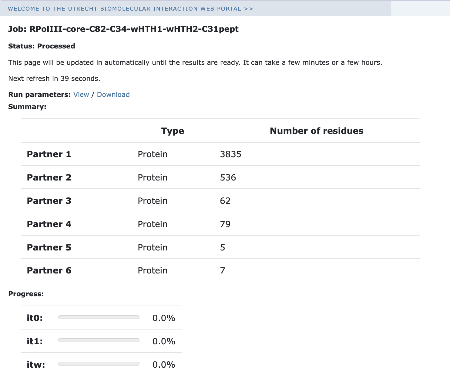
Your run will first be queued but eventually its status will change to “Running” with the page showing the progress of the calculations. The page will automatically refresh and the results will appear upon completion (which can take between 1/2 hour to several hours depending on the size of your system and the load of the server). Since we are dealing here with a large complex, the docking will take quite some time (probably 1/2 day). So be patient. You will be notified by email once your job has successfully completed.
First analysis of the results
Once your run has completed you will be presented with a result page showing the cluster statistics and some graphical representation of the data. If you are using course credentials the number of models generated will have been decreased to allow the runs to complete within a reasonable amount of time. Because of that, the results might not be very good.
We have already performed a full docking run (with 4000/400/400 models generated for the rigid-body docking, semi-flexible and final refinement stages). The full run can be accessed here.
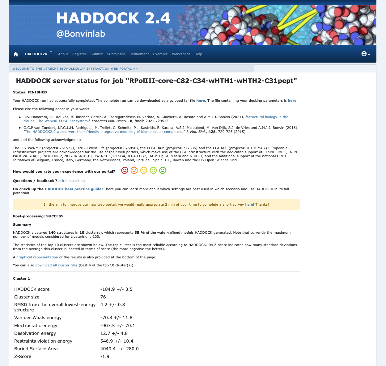
Example result page
Inspect the result page How many clusters are generated?
Note: The bottom of the page gives you some graphical representations of the results, showing the distribution of the solutions for various measures (HADDOCK score, van der Waals energy, …) as a function of the Fraction of Common Contacts and RMSD from the best generated model (the best scoring model). The graphs are interactive and you can turn on and off specific clusters, but also zoom in on specific areas of the plot.
The ranking of the clusters is based on the average score of the top 4 members of each cluster. The score is calculated as:
HADDOCKscore = 1.0 * Evdw + 0.2 * Eelec + 1.0 * Edesol + 0.1 * Eair
where Evdw is the intermolecular van der Waals energy, Eelec the intermolecular electrostatic energy, Edesol represents an empirical desolvation energy term adapted from Fernandez-Recio et al. J. Mol. Biol. 2004, and Eair the AIR (restraints violation) energy. The cluster numbering reflects the size of the cluster, with cluster 1 being the most populated cluster. The various components of the HADDOCK score are also reported for each cluster on the results web page.
Consider the cluster scores and their standard deviations. Is the top ranked cluster significantly better than the second one? (This is also reflected in the z-score).
Visualisation of docked models
Let’s now visualize the various clusters. The result page allows to download individual models, but it also has an option to download all clusters at once. Look for the following sentence, just above the cluster statistics:
You can also download all cluster files (best X of the top 10 cluster(s)).
Download the archive by clicking on the link and unpack it
Start PyMOL and load each cluster representative (clusterX_1.pdb):
File menu -> Open -> select cluster1_1.pdb
Repeat this for each cluster.
Note: If using the command line, all clusters can be loaded easily in one command:
Once all files have been loaded, type in the PyMOL command window:
Let’s then superimpose all models on chain A of the first cluster:
alignto cluster1_1 and chain A
This will align all clusters on chain A (PolIII-core), maximizing the differences in the orientation of the other chains. Be patient as given the size of the system this might take a bit of time…
Note: You can also open in PyMol a session in which the models have already been fitted. Open for this the strategy1-clusters.pse file found in the docking/strategy1-RNA-PolIII-core-C82-C34-wHTHs-C31pept_summary directory
Note: You can turn on and off a cluster by clicking on its name in the right panel of the PyMOL window.
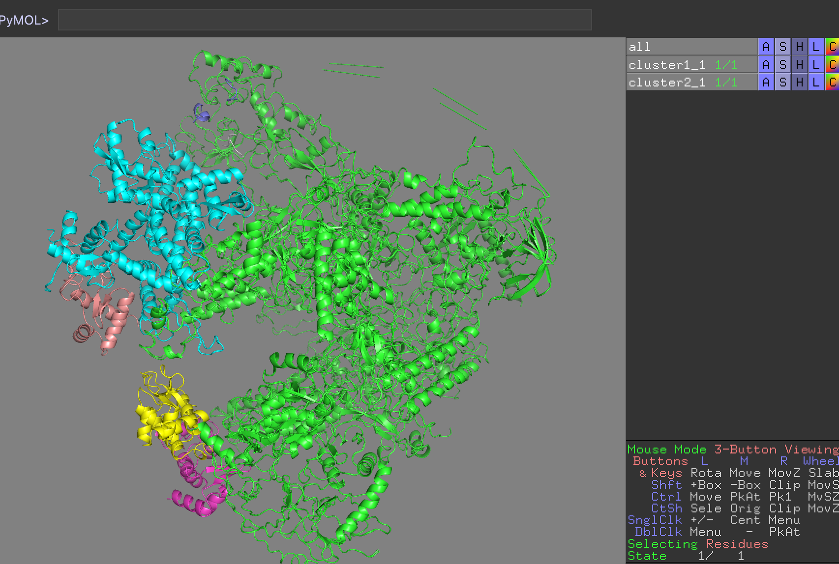
Reminder: ChainA corresponds to PolIII-core (green), B to C82 (blue), C to C34 wHTH1 (magenta), D to C34 wHTH2 (yellow), F and G (wheat and …) to C31.
See PyMol view:
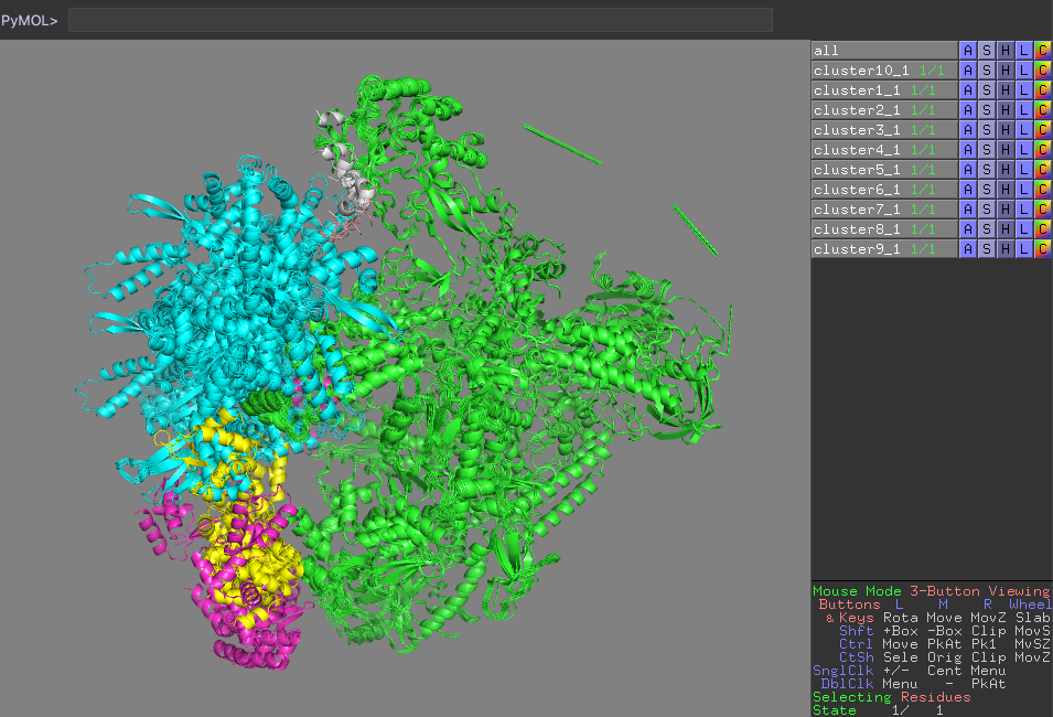
PyMol view of the various clusters, superimposed on PolIII core
Which domain is the best defined over the various clusters?
Which domain is the worst defined over the various clusters?
Satisfaction of cross-link restraints
Let’s now check if the solutions actually fit the cross-links we defined.
Start a new PyMOL session and load as described above the model you want to analyze, e.g. the best model of the top
ranking cluster, cluster1_1.pdb.
Analysing the cross-links defining the position of the C82 domain
In the PyMOL command window type:
This will draw lines between the connected atoms and display the corresponding Euclidian distance. Objects are created in the left panel with their name corresponding to the cross-link and its associated maximum distance.
Inspect the various cross-link distances.
Is the model satisfying the cross-link restraints?
If not, which ones are not satistified?
See answer:
Several cross-links for C82 are heavily violated with distances betweem 38 and ~50A. Clearly this model does not stastify all crosslinks. Check the restraint energy of the various clusters and examine if the one with the best (lowest) restraint energy fits the cross-links better.
Note that the reported distances are Euclidian distances. In reality, the cross-linker will have to follow the surface of the molecule which might results in a longer effective distance. A proper comparison would require calculating the surface distance instead. Such an analysis can be done with the XWalk or jwalk software.
Analysing the cross-links defining the position of the C34 wHTH1 domain
You can first hide the distances shown for C82 by unselecting them in the menu on the right side of the window. Alternatively delete them in PyMol by typing:
In the PyMOL command window type:
Inspect the various cross-link distances.
Is the model satisfying the cross-link restraints?
If not, which ones are not satistified?
See answer:
In the case of C34 wHTH1, all cross-links are satisfied.
Analysing the cross-links defining the position of the C34 wHTH2 domain
You can first hide the distances shown for C82 by unselecting them in the menu on the right side of the window. Alternatively delete them in PyMol by typing:
In the PyMOL command window type:
Inspect the various cross-link distances.
Is the model satisfying the cross-link restraints?
If not, which ones are not satistified?
See answer:
In the case of C34 wHTH2, all cross-links are satisfied.
Analysing the cross-links defining the position of the C31 peptides
You can first hide the distances shown for C34 by unselecting them in the menu on the right side of the window. Alternatively delete them in PyMol by typing:
In the PyMOL command window type:
Inspect the various cross-link distances.
Is the model satisfying the cross-link restraints?
If not, which ones are not satistified?
See answer:
As for C82, there are heavily violated cross-links with distances up to ~50Å, especially the one connecting C31 to C82 (already seen when analysing the fit of the C82 cross-links).
Fitting the docking models into low resolution cryo-EM maps
We will now fit the models we obained into the unpublished 9Å resolution cryo-EM map for the RNA Polymerase III apo state. For this we will use the UCSF Chimera software.
For this open the PDB file of the cluster you want to fit and the EM map PolIII_9A.mrc (available in the cryo-EM directory).
UCSF Chimera Menu → File → Open… → Select the file
Repeat this for each file. Chimera will automatically guess their type.
If you want to use the Chimera command-line instead, you need to first display it:
UCSF Chimera Menu → Favorites → Command Line
and type:
open /path/to/clusterX_1.pdb open /path/to/PolIII_9A.mrc
In the Volume Viewer window, the middle slide bar provides control on the
value at which the isosurface of the density is shown. At high values, the
envelope will shrink while lower values might even display the noise in the map.
In the same window, you can click on Center to center the view on all visible molecules and the density.
We will first make the density transparent, in order to be able to see the fitted structure inside:
Within the Volume Viewer window click on the gray box next to Color
This opens theColor Editor window.
An extra slider bar appears in the box called A, for the alpha channel.
Set the alpha channel value to around 0.6.
In order to distinguish the various chains we can color the structure by chain. For this: Chimera menu -> Tools -> Depiction -> Rainbow Select the option to color by chain and click the Apply button
In order to perform the fit, we will use the Command Line more:
UCSF Chimera Menu → Favorites → Command Line
Also open the Model Panel to know the ID of the various files within Chimera:
UCSF Chimera Menu → Favorites → Model Panel
Note the number of the cluster model you upload and of the cryo-EM map (e.g. if you loaded first the PDB file, it must have model #0 and the map is #1). Then, in the Command Line interface type:
This generate a 9Å map from the PDB model we uploaded with ID #3. The next command then performs the fit of this map onto the experimental cryo-EM map:
fitmap #1 #2 search 100
close #2
When the fit completes, a window will appear showing the fit results in terms of correlation coefficients. Note the value for the cluster you selected.
You also try to improve further the fit: UCSF Chimera Menu → Tools → Volume Data -> Fit in Map
Click the Options button Select the Use map simulated from atoms and set the Resolution to 9 Click on Update and note the correlation value Click on Fit and check if the correlation does improve
You can repeat this procedure for the various clusters and try to find out which solution best fits the map. In case you upload multiple models simultaneously, make sure to use the correct model number in the above commands (check the Model Panel window for this).
Which model gives the best fit to the EM map?
What is the best correlation coefficient obtained?
Note: In the cryo-EM directory of the downloaded data you will find a Python script that can be used to fit a structure
into an EM map using Chimera from the command line. Here is an example of how to run it for the CGref model assuming you
are in the docking/strategy1-RNA-PolIII-core-C82-C34-wHTHs-C31pept_summary directory (if not do correct the path to the CCalculate script and the EM map):
The last number in the command is the number of fittings tried from different random positions. The best fit value will be reported.
View the correlation coefficients calculated with the CCcalculate script of the various clusters:
    cluster1_1.pdb :  0.8939
    cluster2_1.pdb :  0.8957
    cluster3_1.pdb :  0.9225
    cluster4_1.pdb :  0.8931
    cluster5_1.pdb :  0.8200
    cluster6_1.pdb :  0.8193
    cluster7_1.pdb :  0.8085
    cluster8_1.pdb :  0.8959
    cluster9_1.pdb :  0.8941
    cluster10_1.pdb : 0.9143
It looks like this strategy was not able to generate models that fullfil the cross-link restraints (or those restraints are possibly problematic/false positives). In the following we will explore an alternate strategy that will first make use of the cryo-EM data to position the largest components into the map and then dock the remaining models.
Strategy 2): Modelling the complex by docking with cross-links only, using as starting conformations the models fitted into the cryo-EM map
In this alternative strategy we will start by fitting the largest components (core and C82) into the 9Å cryo-EM map using our PowerFit web server. This fitted models will then be used as input for the docking with cross-links, keeping those fixed at their original position.
Introduction to PowerFit
PowerFit is a software developed in our lab to fit atomic resolution structures of biomolecules into cryo-electron microscopy (cryo-EM) density maps. PowerFit performs a rigid body fitting, calculating the cross-correlation, a common measure of the goodness-of-fit, between the atomic structure and the density map. It performs a systematic 6-dimensional scan of the three translational and three rotational degrees of freedom. In short, PowerFit will try to systematically fit the structure in different orientations at every position in the map and calculate a cross-correlation score for each of them.
PowerFit is open-source and available for download from our Github repository. To facilitate its use, we have developed a web portal for it.
The server makes use of either local resources on our cluster, using the multi-core version of the software, or GPGPU-accelerated grid resources of the EGI to speed up the calculations. It only requires a web browser to work and benefits from the latest developments in the software, based on a stable and tested workflow. Next to providing an automated workflow around PowerFit, the web server also summarizes and higlights the results in a single page including some additional postprocessing of the PowerFit output using UCSF Chimera.
For more details about PowerFit and its usage we refer to a related online tutorial.
Fitting PolIII-core and C82+C34wHTH3 into the 9Å cryo-EM map
To run PowerFit, go to
https://alcazar.science.uu.nl/services/POWERFIT
On this page, you will find the most relevant information about the server as well as the links to the local and grid versions of the portal’s submission page.
Click on the “Submit” menu to access the input form:
Complete the form by filling the required fields and selecting the respective files (most browsers should also support dragging the files onto the selection button):
Cryo-EM map → PolIII_9A.mrc Map resolution → 9.0 Atomic structure → A_PolIII-5fja-core.pdb Rotational angle interval → 10.0
Once the fields have been filled in you can submit your job to our server by clicking on “Submit” at the bottom of the page.
If the input fields have been correctly filled you should be redirected to a status page displaying a pop-up message indicating that your run has been successfully submitted. While performing the search, the PowerFit web server will update you on the progress of the job by reloading the status page every 30 seconds.
For convenience, we have already provided pre-calculated results in the cryo-EM/powerfit-PolIII-core directory in the data downloaded for this tutorial.
The fit_1.pdb file corresponds to the top solution predicted by PowerFit. You can inspect it and see how well it fits into the cryo-EM map
using Chimera with its Volume -> Fit in Map tool (see instructions above).
Repeat the above procedure, but this time for the C82+C34wHTH3 AlphaFold model (BE_C82-C34-wHTH3-alphafold-trimmed.pdb).
Pre-calculated results are available in the powerfit-PolIII-core/ and cryo-EM/powerfit-PolIII-C82-C34-wHTH3 directories.
Refining the fit in Chimera
Let’s see how well did PowerFit perform in fitting and try to further optimize the fit using Chimera.
UCSF Chimera Menu → File → Open… → Select the cryo-EM/powerfit-PolIII-core/fit_1.pdb UCSF Chimera Menu → File → Open… → Select the cryo-EM/powerfit-PolIII-C82-C34-wHTH3/fit_1.pdb UCSF Chimera Menu → File → Open… → Select the cryo-EM/PolIII_9A.mrc
In the Volume Viewer window, the middle slide bar provides control on the
value at which the isosurface of the density is shown. At high values, the
envelope will shrink while lower values might even display the noise in the map.
In the same window, you can click on Center to center the view on all visible molecules and the density.
First make the density transparent, in order to be able to see the fitted structure inside:
Within the Volume Viewer window click on the gray box next to Color Set the alpha channel value to around 0.6.
In order to distinguish the various chains color the structure by chain:
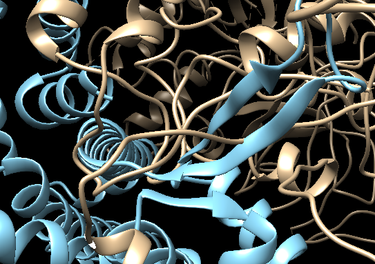
The two molecules were fitted separately into the map, which can cause clashes at the interface. Inspect the interface (first turn off the map by clicking on the “eye” in the Volume Viewer window).
Can you identify possible problematic areas of the interface?
See solution:
There are clearly several regions where the two molecules are clashing.
Now let’s check the quality of the fit and try to improve the fit in Chimera:
UCSF Chimera Menu → Tools → Volume Data -> Fit in Map Click the Options button Select the Use map simulated from atoms and set the Resolution to 9 Click on Update and note the correlation value Click on Fit and check if the correlation does improve Has the quality of the fit measured bu correlation coefficient improved?
Repeat this procedure using the second molecule (fit_1#1) corresponding to the C82+C34wHTH3 model.
What about the clashes? Is the fit between core and C82 better in terms of clashes?
See solution:
The fit in chimera has clearly removed some of the chain clashes, but there are still regions where the two molecules are clashing (especially considering we don't visualize the side-chains.
Do save the fitted molecules:
This will save both molecules into one PDB file as multimodel file (i.e. with MODEL/ENDMDL statements). In order to use this file for refinement with HADDOCK we need to merge two two models into one. This can be done either manually by editing the PDB file and removing all MODEL/ENDMDL statements, or using our PDB-tools webserver.
To use PDB-tools click on the above link.
Click on Submit in the top panel.
As pre-processing option select: pdb_splitmodel and click on the + button to add it to the workflow
As post-processing option select: pdb_merge and click on the + button to add it to the workflow
Download the merged_1.pdb file, we will use it as input for refinement in HADDOCK
A pre-processed PDB file is already available on disk: PolIII-core-C82-C34-wHTH3-chimera-fitted-merged.pdb.
Refining the interface of the cryo-EM fitted models with HADDOCK
To refine the fitted models, we can use the HADDOCK2.4 refinement interface which offers different options to refine a complex. Their performance to refine complexes obtained by individually fitting molecules into low to medium resolution EM maps is described in:
- T Neijenhuis, S.C. van Keulen and A.M.J.J. Bonvin. Interface Refinement of Low-to-Medium Resolution Cryo-EM Complexes using HADDOCK2.4. Structure 30, 476-484 (2022).
Considering the size of the system we recommend in this case either the default water refinement or the coarse-grained refinement.
Connect to the HADDOCK2.4 refinement interface of the HADDOCK web server.
-
Step 1: Define a name for your refinement run, e.g. PolIII-core-C82-refine.
-
Step 2: Input the PDB file of the complex.
- Step 3: Choose the refinement protocol
What protocol do you want to use? -> Coarse-grained refinement
Considering the size of the system, the coarse-grained refinement is much more efficient in this case.
The server will process the PDB files and recognize the number of chains and their type.
- Step 4: Submission
As nothing need to be changed further click on Submit
Note: The refinement interface allows to refine complexes consisting of various number of chains, but also single molecules. Also an ensemble of conformations can be submitted.
The result page of such a refinement can be found:
How do the correlation coefficient of the unrefined and refined models compare?
View the pre-calculated correlation coefficients for the various models:
     PolIII-core-C82-C34-wHTH3-chimera-fitted-merged.pdb:  0.9446
     PolIII-core-C82-C34-wHTH3-chimera-fitted-watref.pdb:  0.9336
     PolIII-core-C82-C34-wHTH3-chimera-fitted-CGref.pdb:   0.9496
Note: In the cryo-EM directory of the downloaded data you will find a Python script that can be used to fit a structure into an EM map using Chimera from the command line. Assuming that you are in the pre-calculatedcryo-EM directory:
The last number in the command is the number of fittings tried from different random positions. The best fit value will be reported.
View an example output of the CCcalculate script:
RNA-Pol-III-2022/cryo-EM> chimera --nogui --script "CCcalculate.py PolIII-core-C82-C34-wHTH3-chimera-fitted-CGref.pdb PolIII_9A.mrc 9 10"
Opening PolIII-core-C82-C34-wHTH3-chimera-fitted-CGref.pdb...
...

Model 0 (PolIII-core-C82-C34-wHTH3-chimera-fitted-CGref.pdb) appears to be a protein without secondary structure assignments.
Automatically computing assignments using 'ksdssp' and parameter values:
  energy cutoff -0.5
  minimum helix length 3
  minimum strand length 3
Use command 'help ksdssp' for more information.

Computing secondary structure assignments...
Computed secondary structure assignments (see reply log)
reading PolIII_9A.mrc 2.8 Mb 0%
Done reading PolIII_9A.mrc
reading PolIII_9A.mrc 178 Mb 0%
Done reading PolIII_9A.mrc
Fit 1 of 10
Fit 2 of 10
Fit 3 of 10
Fit 4 of 10
Fit 5 of 10
Fit 6 of 10
Fit 7 of 10
Fit 8 of 10
Fit 9 of 10
Fit 10 of 10
Fit search: finished
Found 9 unique fits from 10 random placements having fraction of points inside contour >= 0.100 (10 of 10).

Correlations and times found:
	0.952 (1), 0.8203 (1), 0.8133 (1), 0.8103 (2), 0.8049 (1), 0.8041 (1), 0.8009 (1), 0.7976 (1), 0.7753 (1)

Best fit found:
Fit map molmap PolIII-core-C82-C34-wHTH3-chimera-fitted-CGref.pdb res 9 in map PolIII_9A.mrc using 33394 points
  correlation = 0.952, correlation about mean = 0.595, overlap = 208
  steps = 328, shift = 49.3, angle = 31.6 degrees
Position of molmap PolIII-core-C82-C34-wHTH3-chimera-fitted-CGref.pdb res 9 (#0.1) relative to PolIII_9A.mrc (#1) coordinates:
  Matrix rotation and translation
     0.10322358  -0.51111512  -0.85329141 185.59573168
     0.45569008  -0.73824752   0.49733002 190.85526186
    -0.88413316  -0.44017262   0.15670554 189.33240076
  Axis  -0.69596127   0.02289558   0.71771422
  Axis point 133.17124957 144.56295228   0.00000000
  Rotation angle (degrees) 137.65984172
  Shift along axis  11.08885675

correlation = 0.9496, corr about mean = 0.5599
Correlation between molmap PolIII-core-C82-C34-wHTH3-chimera-fitted-CGref.pdb res 9 and PolIII_9A.mrc = 0.9496, about mean = 0.5599
Note that we also performed the fitting using only the C82 model. Results can be found on disk (powerfit-PolIII-C82 directory). Analysis in Chimera reveals unaccounted density in proximity of the C82 domain where the C34 wHTH3 domain is found in the analysis performed above, which gives confidence in the C82+C34wHTH3 model obtained with AlphaFold-multimer.
Checking the agreement of the refined cryo-EM fitted models with the cross-links
Let’s now check if the EM-fitted model of core+C82+C34wHTH3 fits the two cross-links we have between those domains.
Start a new PyMOL session and load as described above PolIII-core-C82-C34-wHTH3-chimera-fitted-CGref.pdb.
In the PyMOL command window type:
Inspect the various cross-link distances.
Is the model satisfying the cross-link restraints?
If not, which one(s) is(are) not satistified?
See answer:
Both cross-links are violated, but especially the one between core residue 5394 and C82 residue 472 (~70Å!). The EM fitting solution for C82+C34wHTH3 was well defined according to PowerFit. There seems thus to be discrepancy between the EM and MS data. Another explanation could be conformational changes in the structures that are not accounted for in our modelling.
Setting up the full docking run using the cryo-EM fitted and refined core and C82 domains
We will now repeat the steps from the the first HADDOCK run submission, with as difference that we will use the PowerFit/Chimera, HADDOCK-refined structures of PolIII core and C82. Those will be kept fixed in their original positions for the initial rigid-body docking stage.
Connect to the HADDOCK2.4 interface of the HADDOCK web server.
Submission of structures
-
Step 1: Define a name for your docking run, e.g. RPolIII-EMfit-C34-wHTH1-wHTH2-C31-xlinks.
-
Step 2: Define the number of components, i.e. 7.
-
Step 3: Input the first PDB file.
Which chain to be used? -> A PDB structure to submit -> Browse and select from the cryo-EM directory PolIII-core-C82-C34-wHTH3-chimera-fitted-CGref.pdb Do you want to coarse-grain your molecule? -> turn on Fix molecule at its original position during it0? -> turn on
- Step 4: Input the second protein PDB files.
Which chain to be used? -> B PDB structure to submit -> Browse and select from the cryo-EM directory PolIII-core-C82-C34-wHTH3-chimera-fitted-CGref.pdb Do you want to coarse-grain your molecule? -> turn on Fix molecule at its original position during it0? -> turn on
- Step 5: Input the third protein PDB files.
PDB structure to submit -> Browse and select from the input-pdbs directory C_C34_wHTH1-alphafold.pdb
- Step 6: Input the fourth protein PDB files.
PDB structure to submit -> Browse and select from the input-pdbs directory D_C34_wHTH2-alphafold.pdb
- Step 7: Input the fifth protein PDB files.
Which chain to be used? -> E PDB structure to submit -> Browse and select from the cryo-EM directory PolIII-core-C82-C34-wHTH3-chimera-fitted-CGref.pdb Do you want to coarse-grain your molecule? -> turn on Fix molecule at its original position during it0? -> turn on
- Step 8: Input the sixth protein PDB files.
- Step 9: Input the fifth protein PDB files.
- Step 10: Click on the “Next” button at the bottom left of the interface.
Definition of restraints
If everything went well, the interface window should have updated itself and it should show the list of residues for molecules 1 and 2.
-
Step 11: Instead of specifying active and passive residues, we will supply restraint files to HADDOCK. No further action is required in this page, so click on the “Next” button at the bottom of the Input parameters window, which proceeds to the Distance Restraint menu of the Docking Parameters window.
-
Step 12: Upload the cross-link restraints file
Other docking settings and job submission
In the same page as where restraints are provided you can modify a large number of docking settings.
- Step 13: Unfold the sampling parameters menu.
Here you can change the number of models that will be calculated, the default being 1000/200/200 for the three stages of HADDOCK (see HADDOCK General Concepts. When docking multiple subunits, depending on the amount of information available to guide the docking, it is recommended to increase the sampling. For this tutorial we will use 4000/400/400 (but if you are using course accounts, this will be automatically downsampled to 250/50/50).
Number of structures for rigid body docking -> 4000
Number of structures for semi-flexible refinement -> 400
Number of structures for the final refinement -> 400
Number of structures to analyze -> 400
When docking only with interface information (i.e. no specific distances), we are systematically sampling the 180 degrees rotated solutions for each interface, minimizing the rotated solution and keeping the best of the two in terms of HADDOCK score. Since here we are using rather specific distance restraints, we can turn off this option to save time.
Sample 180 degrees rotated solutions during rigid body EM -> turn off
- Step 14: Unfold the clustering parameters menu.
The default clustering methods in Fraction of Native Contacts (FCC). Since we are dealing with multiple interfaces, to have a better discrimination of solutions we will increase the cutoff to 0.75.
- Step 15: Submission.
We are now ready to submit the docking run. Scroll to the bottom of the page.
Click on the “Submit” button at the bottom left of the interface.
Upon submission you will be presented with a web page which also contains a link to the previously mentioned haddockparameter file as well as some information about the status of the run.
Your run will first be queued but eventually its status will change to “Running” with the page showing the progress of the calculations. The page will automatically refresh and the results will appear upon completion (which can take between 1/2 hour to several hours depending on the size of your system and the load of the server). Since we are dealing here with a large complex, the docking will take quite some time (probably 1/2 day). So be patient. You will be notified by email once your job has successfully completed.
First analysis of the docking results
Once your run has completed you will be presented with the result page. You can also access a pre-calculated run following the docking scenario just described from the following link.
Inspect the result page How many clusters are generated? Consider the cluster scores and their standard deviations. If there is more than one cluster, is the top ranked cluster significantly better than the second one? (This is also reflected in the z-score). Compare the score and the various energy terms of the best cluster and the best cluster obtained using Strategy 1) using only cross-links. Which strategy leads to better scores/energies?
Visualisation of docked models
Let’s now visualize the various clusters. Download all clusters at once and unpack the archive.
Start PyMOL and load each cluster representative (clusterX_1.pdb):
File menu -> Open -> select cluster1_1.pdb
Repeat this for each cluster.
Note: If using the command line, all clusters can be loaded easily in one command:
Once all files have been loaded, type in the PyMOL command window:
Let’s then superimpose all models on chain A of the first cluster:
alignto cluster1_1 and chain A
This will align all clusters on chain A (PolIII-core), maximizing the differences in the orientation of the other chains. Be patient as given the size of the system this might take a bit of time…
Note: You can also open in PyMol a session in which the models have already been fitted. Open for this the strategy2-clusters.pse file found in the docking/strategy2-RNA-PolIII-core-C82-C34-wHTHs-C31pept_summary directory
Reminder: ChainA corresponds to PolIII-core (green), B to C82 (blue), C to C34 wHTH1 (magenta), D to C34 wHTH2 (yellow), E to C34 wHTH3 (wheat) and F and G (violet and gray) to C31.
See PyMol view:
PyMol view of the various clusters, superimposed on PolIII core
Which domain is the best defined over the various clusters?
Which domain is the worst defined over the various clusters?
How different are the solutions compared to those of Strategy1?
Satisfaction of cross-link restraints
Let’s now check if the solutions actually fit the cross-links we defined.
Start a new PyMOL session and load as described above the model you want to analyze, e.g. the best model of the top
ranking cluster, clusterX_1.pdb.
Analysing the cross-links defining the position of the C82 domain
In the PyMOL command window type:
This will draw lines between the connected atoms and display the corresponding Euclidian distance. Objects are created in the left panel with their name corresponding to the cross-link and its associated maximum distance.
Inspect the various cross-link distances.
Is the model satisfying the cross-link restraints?
If not, which ones are not satistified?
See answer:
The fit is better than in strategy 1, but thre is still one heavily violated cross-link between resid 472 of C82 and resid 5394 of the core. This might well be a false positive. It was not detected by DISVIS because the analysis is only performed for pair of domain and it can be satisfied, while when considering all molecules and all cross-links it can not.
Analysing the cross-links defining the position of the C34 wHTH1 domain
You can first hide the distances shown for C82 by unselecting them in the menu on the right side of the window. Alternatively delete them in PyMol by typing:
In the PyMOL command window type:
Inspect the various cross-link distances.
Is the model satisfying the cross-link restraints?
If not, which ones are not satistified?
See answer:
In the case of C34 wHTH1, all cross-links are satisfied.
Analysing the cross-links defining the position of the C34 wHTH2 domain
You can first hide the distances shown for C82 by unselecting them in the menu on the right side of the window. Alternatively delete them in PyMol by typing:
In the PyMOL command window type:
Inspect the various cross-link distances.
Is the model satisfying the cross-link restraints?
If not, which ones are not satistified?
See answer:
In the case of C34 wHTH2, all cross-links are satisfied.
Analysing the cross-links defining the position of the C31 peptides
You can first hide the distances shown for C34 by unselecting them in the menu on the right side of the window. Alternatively delete them in PyMol by typing:
In the PyMOL command window type:
Inspect the various cross-link distances.
Is the model satisfying the cross-link restraints?
If not, which ones are not satistified?
See answer:
All cross-links are now stastified, including the one with C82 that was not in strategy 1.
Fitting the docking models into low resolution cryo-EM maps
We will now fit the models we obained into the unpublished 9Å resolution cryo-EM map for the RNA Polymerase III apo state. For this we will use the UCSF Chimera software.
For this open the PDB file of the cluster you want to fit and the EM map PolIII_9A.mrc (available in the cryo-EM directory).
UCSF Chimera Menu → File → Open… → Select the file
Repeat this for each file. Chimera will automatically guess their type.
If you want to use the Chimera command-line instead, you need to first display it:
UCSF Chimera Menu → Favorites → Command Line
and type:
open /path/to/clusterX_1.pdb open /path/to/PolIII_9A.mrc
In the Volume Viewer window, the middle slide bar provides control on the
value at which the isosurface of the density is shown. At high values, the
envelope will shrink while lower values might even display the noise in the map.
In the same window, you can click on Center to center the view on all visible molecules and the density.
We will first make the density transparent, in order to be able to see the fitted structure inside:
Within the Volume Viewer window click on the gray box next to Color
This opens theColor Editor window.
An extra slider bar appears in the box called A, for the alpha channel.
Set the alpha channel value to around 0.6.
In order to distinguish the various chains we can color the structure by chain. For this: Chimera menu -> Tools -> Depiction -> Rainbow Select the option to color by chain and click the Apply button
In order to perform the fit, we will use the Command Line more:
UCSF Chimera Menu → Favorites → Command Line
Also open the Model Panel to know the ID of the various files within Chimera:
UCSF Chimera Menu → Favorites → Model Panel
Note the number of the cluster model you upload and of the cryo-EM map (e.g. if you loaded first the PDB file, it must have model #0 and the map is #1). Then, in the Command Line interface type:
This generate a 9Å map from the PDB model we uploaded with ID #3. The next command then performs the fit of this map onto the experimental cryo-EM map:
fitmap #1 #3 search 100
close #3
When the fit completes, a window will appear showing the fit results in terms of correlation coefficients. Note the value for the cluster you selected.
You also try to improve further the fit: UCSF Chimera Menu → Tools → Volume Data -> Fit in Map
Click the Options button Select the Use map simulated from atoms and set the Resolution to 9 Click on Update and note the correlation value Click on Fit and check if the correlation does improve
You can repeat this procedure for the various clusters and try to find out which solution best fits the map. In case you upload multiple models simultaneously, make sure to use the correct model number in the above commands (check the Model Panel window for this).
Which model gives the best fit to the EM map?
What is the best correlation coefficient obtained?
Note: In the cryo-EM directory of the downloaded data you will find a Python script that can be used to fit a structure
into an EM map using Chimera from the command line. Here is an example of how to run it for the CGref model assuming you
are in the docking/strategy2_RNA-PolIII-core-C82-C34-C31pept_summary directory (if not do correct the path to the CCalculate script and the EM map):
The last number in the command is the number of fittings tried from different random positions. The best fit value will be reported.
View the correlation coefficients calculated with the CCcalculate script of the various clusters:
    cluster1_1.pdb :  0.9435
    cluster1_2.pdb :  0.9439
    cluster1_3.pdb :  0.9458
    cluster1_4.pdb :  0.9434
    cluster2_1.pdb :  0.9456
    cluster2_2.pdb :  0.9425
    cluster2_3.pdb :  0.9415
    cluster2_4.pdb :  0.9504
See solution:
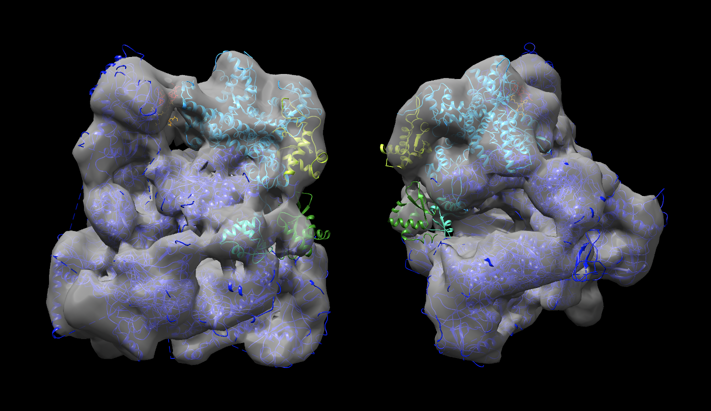
Strategy 2, consisting of first fitting the largest domains into the map and using those as starting point for the docking leads to a better fit in the EM map (correlation 0.9504). Comparing the two sets of solutions, one can clearly see that C82 fits much better into the density. The C34 wHTH3 domain (yellow) also nicely fit into the density. The other two C34 domains (green and cyan are found in a region where some density starts to appear seen when playing with the density level, which might indicate some disorder / conformational variability.
Conclusions
We have demonstrated the use of cross-linking data from mass spectrometry for guiding the docking process in HADDOCK. The results show that it is not straightforward to satisfy all cross-links. In the original work of Ferber et al. 2016 from which the cross-links were taken, many cross-links remained violated. See for example Suppl. Table 5 in the corresponding supplementary material. It is also possible that the cross-linking experiments might have captured transient or non-native interactions.
Our modelling here was based partially on models (from AlphaFold), which brings another level of complexity. Clearly some domains show much more variability in their positions, which might explain why they are not seen in the cryo-EM density.
And finally, using the cryo-EM data to pre-orient molecules prior to docking seems to be a better strategy in this particular case.
Alternative runs
Try to identify from the runs described in this tutorial the heavily violated cross-links and remove them from the restraints list. Repeat the docking and check if this affects the position of the various domains (especially for Strategy 1).
Congratulations!
Thank you for following this tutorial. If you have any questions or suggestions, feel free to contact us via email, or post your question to
our HADDOCK forum hosted by the
![]() Center of Excellence for Computational Biomolecular Research.
Center of Excellence for Computational Biomolecular Research.