

Modelling a homo-oligomeric complex from MS cross-links
This tutorial consists of the following sections:
- Introduction
- Setup/Requirements
- Inspecting the data
- Visualizing the accessible interaction space with DisVis
- Analysing the DisVis results
- Modelling the symmetrical homomeric complex using HADDOCK
- Analysing the docking results
- Your report
- Bonus: Predicting the oligomeric state with AlphaFold2
- Bonus II: Predicting the oligomeric state with AlphaFold3
Introduction
In this tutorial, your task is to determine the oligomeric state of a homomeric symmetrical complex and model its 3D structure, based on cross-linking data obtained by mass spectrometry. Note that for the purpose of this tutorial we are using simulated data that would correspond to rather short cross-linkers that are not amino-acid specific. We are also assuming that all detected cross-links are highly reliable, i.e. there are no false positives in our data. (This differs thus from our DisVis Webserver Tutorial in which you first have to identify false positives).
You will first use our DisVis web server to analyse the data and visualise the accessible interaction space defined by the cross-links. Based on those results you should then make a choice about the putative oligomeric state of the complex (e.g. homodimer, homotrimer, homotetramer,…) and then try to model its 3D structure using our HADDOCK2.4 web portal. This means defining the cross-links as distance restraints to guide the docking and imposing symmetry restraints to generate the proper homomeric complex. Those two aspects are described in two related online tutorials:
-
HADDOCK2.4 MS cross-links tutorial: A tutorial demonstrating the use of cross-linking data from mass spectrometry to guide the docking in HADDOCK.
-
HADDOCK2.4 ab-initio, multi-body symmetrical docking tutorial: A tutorial demonstrating multi-body docking with HADDOCK using its ab-initio mode with symmetry restraints.
For this tutorial we will make use of the HADDOCK2.4 webserver.
A description of DisVis and of the HADDOCK2.4 web server can be found in the following publications:
-
G.C.P. van Zundert, M. Trellet, J. Schaarschmidt, Z. Kurkcuoglu, M. David, M. Verlato, A. Rosato and A.M.J.J. Bonvin. The DisVis and PowerFit web servers: Explorative and Integrative Modeling of Biomolecular Complexes.. J. Mol. Biol.. 429(3), 399-407 (2016).
-
G.C.P van Zundert and A.M.J.J. Bonvin. DisVis: Quantifying and visualizing accessible interaction space of distance-restrained biomolecular complexes. Bioinformatics 31, 3222-3224 (2015).
- R.V. Honorato, M.E. Trellet, B. Jiménez-García, J.J. Schaarschmidt, M. Giulini, V. Reys, P.I. Koukos, J.P.G.L.M. Rodrigues, E. Karaca, G.C.P. van Zundert, J. Roel-Touris, C.W. van Noort, Z. Jandová, A.S.J. Melquiond and A.M.J.J. Bonvin The HADDOCK2.4 web server: A leap forward in integrative modelling of biomolecular complexes. Nature Protoc, 19, 3219–3241 DOI: 10.1038/s41596-024-01011-0 (2024)
Further, multi-body docking and the use of symmetry restraints is described in the following paper:
- E. Karaca, A.S.J. Melquiond, S.J. de Vries, P.L. Kastritis and A.M.J.J. Bonvin. Building macromolecular assemblies by information-driven docking: Introducing the HADDOCK multi-body docking server. Mol. Cell. Proteomics, 9, 1784-1794 (2010).
Throughout the tutorial, coloured text will be used to refer to questions, instructions, and PyMOL commands.
This is a question prompt: Answer it! (This will be part of the report you should submit) This is an instruction prompt: follow it! This is a PyMOL prompt: write this in the PyMOL command line prompt!
Setup/Requirements
In order to follow this tutorial you only need a web browser, a text editor and PyMOL (freely available for most operating systems) on your computer in order to visualize the input and output data.
Further, the required data to run this tutorial should be aquired from this download link here. Once downloaded, make sure to unzip the archive.
Inspecting the data
Let us first inspect the available data, namely the structure of the monomeric protein and the cross-links.
The downloaded data contain 5 PDB files, which are identical copies of the same monomeric protein, but with different chainIDs (A,B,C,D,E). Note that this does not imply the solution is a pentamer per se…
The detected cross-links are between the following residues:
# cross-links
Residue  40 <-> 252
Residue  90 <-> 176
Residue 135 <-> 158
Residue 161 <-> 132
In principle, since we are dealing with a homomeric complex, we don’t know if those cross-links are intra- or intermolecular. Based on the cross-linking reaction we assume here a maximum distance between CA carbons of 10Å. Let us first inspect the structure and check if those cross-links could be explained by intramolecular links.
Using PyMOL, we will visualize the information from MS.
For this open first the PDB file monomer-A.pdb.
PyMOL Menu → File → Open… → Select the file
If you want to use the PyMOL command-line instead, type the following command:
Highlight the residues involved in cross-links:
as cartoon
select name CA and resid 40+90+135+161+252+176+158+132
show sphere, sele
The CA atoms of those residues are now shown as spheres. Let’s now measure the intramolecular distances corresponding to the detected cross-links:
This creates four objects called dist01…dist04. You toggle them on and off in the right panel by clicking on them. Check the reported distance for each .
In case you do identify a crosslink that could be explained by an intramolecular contact (within the same monomer), exclude it from all steps in the remaining part of this tutorial.
Visualizing the accessible interaction space with DisVis
DisVis is a software we developed that allows you to visualize and quantify the information content of distance restraints between macromolecular complexes. It performs a full and systematic 6 dimensional search of the three translational and rotational degrees of freedom of the two components of a complex to determine the number of solutions consistent with the restraints.
It outputs information about the inconsistent/violated restraints and a density map that represents the center-of-mass position of the scanning chain consistent with a given number of restraints at every position in space.
DisVis requires three input files: two high-resolution atomic structures of the biomolecules to be analysed (monomer-A.pdb and
monomer-B.pdb in this particular case) and a text file containing the list of distance restraints between the two molecules.
The cross-links should be defined according to the following format:
<chainid 1> <resid 1> <atomname 1> <chainid 2> <resid 2> <atomname 2> <mindist> <maxdist>
In this particular case, for the DisVis analysis, we have to duplicate the cross-links given above since we are dealing with a symmetrical homomeric system. This is required since in principle we don’t know from which monomer they originate.
The data you downloaded already contain a text file with the cross-links defined in the proper DisVis format: cross-links.txt
# cross-links
A  40 CA B 252 CA 3.0 10.0
A  90 CA B 176 CA 3.0 10.0
A 135 CA B 158 CA 3.0 10.0
A 161 CA B 132 CA 3.0 10.0
#
# symmetrical cross-links
A 252 CA B  40 CA 3.0 10.0
A 176 CA B  90 CA 3.0 10.0
A 158 CA B 135 CA 3.0 10.0
A 132 CA B 161 CA 3.0 10.0
Q2: Can you rationalize why we are using a lower limit of 3Å between two CA atoms?
We have all input data required to run DisVis. To launch the run go to:
https://wenmr.science.uu.nl/disvis
On this page, you will find the most relevant information about the server.
- Step1: Register to the server
Register for getting access to the web server (or use the credentials provided to you).
You can click on the “Register” menu from any DisVis page and fill the required information. Registration is not automatic but is usually processed within 12h, so be patient.
- Step2: Define the input files and parameters and submit
Click on the “Submit” menu to access the input form.
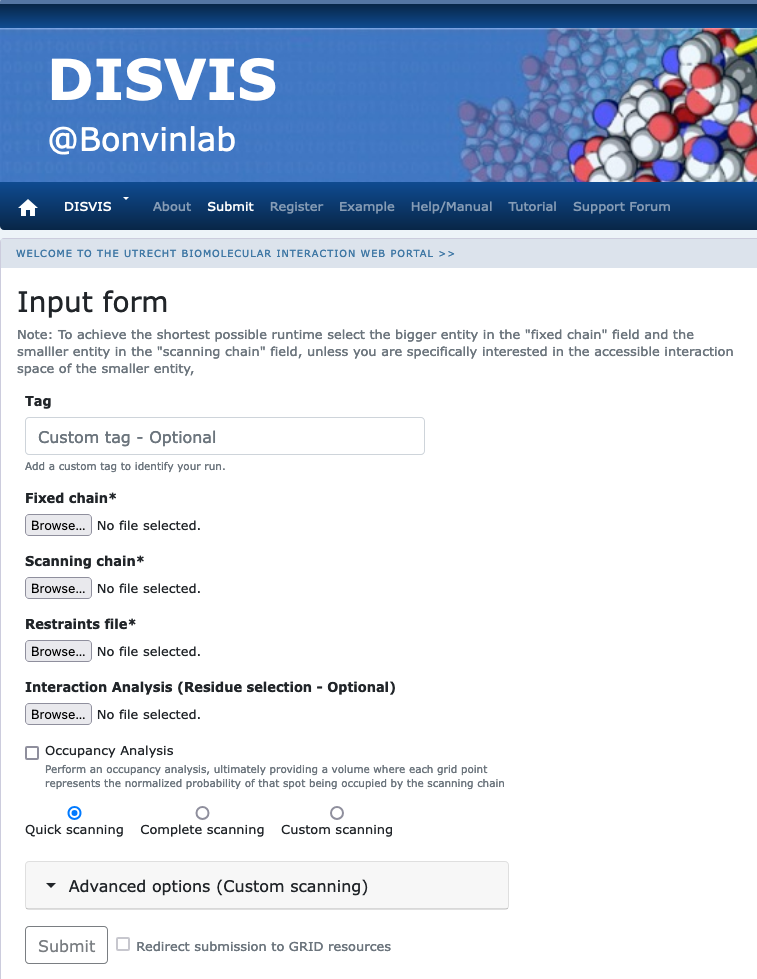
Fixed chain → monomer-A.pdb Scanning chain → monomer-B.pdb Restraints file → cross-links.txt
Once the fields have been filled in, you can submit your job to our server by clicking on “Submit” at the bottom of the page.
If the input fields have been correctly filled you should be redirected to a status page displaying a message indicating that your run has been successfully submitted. While performing the search, the DisVis web server will update you on the progress of the job by reloading the status page every 30 seconds. The runtime of this example case is usually below 5 minutes on our local CPU and grid GPU servers. However the load of the server as well as pre- and post-processing steps might substantially increase the time until the results are available.
The default on the server is to perform a quick scanning grid search (meaning 15.00° rotational sampling and 2.0Å grid) in order to get results in a reasonable time.
You can however choose to perform a complete scanning, which should give more reliable results (9.72° rotational sampling and 1.0Å grid).
Analysing the DisVis results
Web server output
Once your job has completed, and provided you did not close the status page, you will be automatically redirected to the results page (you will also receive an email notification).
See solution
If you don't want to wait for your run to complete, you can access the precalculated results of a run submitted with the same input and complete scanning here.You can also download the corresponding archive here.
The results page presents a summary split into several sections:
Status: In this section you will find a link from which you can download the output data as well as some information about how to cite the use of the portal.Accessible Interaction Space: Here, images of the fixed chain together with the accessible interaction space, in a density map representation, are displayed. Different views of the molecular scene can be chosen by clicking on the right or left part of the image frame. Each set of images matches a specific level of N restraints which corresponds to the accessible interaction space by complexes consistent with at least N restraints. A slider below the image container allows you to change the the number of restraints N and load the corresponding set of images.Accessible Complexes: Summary of the statistics for number of complexes consistent with at least N number of restraints. The statistics are displayed for the N levels, N being the total number of restraints provided in the restraints file (hererestraints.txt)z-Score: For each restraint provided as input, a z-Score is provided, giving an indication of how likely it is that the restraint is a false positive. The higher the score, the more likely it is that a restraint might be a false positive. Putative false positive restraints are only highlighted if no single solution was found to be consistent with the total number of restraints provided. If DisVis finds complexes consistent with all restraints, the z-Scores are still displayed, but should be ignored.Violations: The table in this sections shows how often a specific restraint is violated for all models consistent with a given number of restraints. The higher the violation fraction of a specific restraint, the more likely it is to be a false positive. Column 1 shows the number of consistent restraints N, while each following column indicates the violation fractions of a specific restraint for complexes consistent with at least N restraints. Each row thus represents the fraction of all complexes consistent with at least N restraints that violated a particular restraint. As for the z-Scores, if solutions have been found that are consistent with all restraints provided, this table should be ignored.
Take your time to analyse the output of DisVis and try to answer the following questions.
Looking at the z-Score section, the DisVis output does highlight some restraints as likely false positives.
Remember however that we have full trust in our cross-links.
So we don’t expect any false positives. Look now at the pictures visualising the accessible space in the Accessible Interaction Space section.
Change the value of the slider Current Level (N). Changing its value changes the displayed accessible space, showing the space consistent with N cross-links.
Q4: Do you observe a continuous density?
Now set the Current Level (N) to its maximum value and look at the view from the top of the structure (i.e. looking down the helices) (you can toggle between different views by clicking on the arrows on the side of the picture):
The next step in this tutorial will be to model the complex based on the cross-links and the oligomeric state you think if the correct one from the DisVis analysis.
Modelling the symmetrical homomeric complex using HADDOCK
Our information-driven docking approach HADDOCK has been a consistent top predictor and scorer since the start of its participation in the CAPRI community-wide blind docking experiment. This sustained performance is due, in part, to its ability to integrate experimental data and/or bioinformatics information into the modelling process, and also to the overall robustness of the scoring function used to assess and rank the predictions.
Here we will use HADDOCK in order to model the symmetrical oligomeric state of this complex. In order to drive the docking process we will make use of the following information:
- Knowledge of the stochiometry of the complex (from your above analysis of DisVis results), i.e. how many monomers should we dock?
- Distance restraints based on MS cross-links
- Center-of-mass restraints to bring the subunits together and ensure compact solutions
- Symmetry restraints to define the symmetry of the assembly.
For this you will make use of the docking interface of our HADDOCK web portal. This does require guru level access (provided with course credentials if given to you, otherwise register to the server and request this access level)
Before setting up the docking we need first to generate the distance restraint file for the cross-links in a format suitable for HADDOCK. HADDOCK uses CNS as computational engine. A description of the format for the various restraint types supported by HADDOCK can be found in our Nature Protocol paper, Box 4.
Distance restraints are defined as follows:
assign (selection1) (selection2) distance, lower-bound correction, upper-bound correction
The lower limit for the distance is calculated as: distance minus lower-bound correction and the upper limit as: distance plus upper-bound correction
The syntax for the selections can combine information about:
- chainID -
segidkeyword - residue number -
residkeyword - atom name -
namekeyword.
Other keywords can be used in various combinations of OR and AND statements. Please refer for that to the online CNS manual.
E. g. a distance restraint between the CB carbons of residues 10 and 200 in chains A and B with an allowed distance range between 10 and 20Å would be defined as follows:
assign (segid A and resid 10 and name CB) (segid B and resid 200 and name CB) 20.0 10.0 0.0
A HADDOCK-compatible distance restraint file based on the cross-links defined above for DisVis is already provided in the data you downloaded: crosslinks-restraints.tbl.
It contains the following distance restraints (8 in total):
assign (segid A and resid  40   and name  CA ) (not segid A and resid  252  and name  CA )  10.0 7.0 0.0
assign (segid A and resid  90   and name  CA ) (not segid A and resid  176  and name  CA )  10.0 7.0 0.0
assign (segid A and resid  135  and name  CA ) (not segid A and resid  158  and name  CA )  10.0 7.0 0.0
assign (segid A and resid  161  and name  CA ) (not segid A and resid  132  and name  CA )  10.0 7.0 0.0
assign (segid A and resid  252  and name  CA ) (not segid A and resid   40  and name  CA )  10.0 7.0 0.0
assign (segid A and resid  176  and name  CA ) (not segid A and resid   90  and name  CA )  10.0 7.0 0.0
assign (segid A and resid  158  and name  CA ) (not segid A and resid  135  and name  CA )  10.0 7.0 0.0
assign (segid A and resid  132  and name  CA ) (not segid A and resid  161  and name  CA )  10.0 7.0 0.0
Since we might be docking various numbers of monomers - and we thus don’t know to which monomer a cross-link should be defined,
the above syntax will define distance restraints between the CA atoms of chain A and the corresponding CA atoms of all other chains (the "not segid A" part of the second selection).
Let’s now setup the docking run!
Registration / Login
In order to start the submission, either click on “here” next to the submission section, or click here. To start the submission process, we are prompted for our login credentials. After successful validation of our credentials we can proceed to the structure upload.
Note: The blue bars on the server can be folded/unfolded by clicking on the arrow on the left
Submission and validation of structures
For this we will make us of the HADDOCK 2.4 interface of the HADDOCK web server
-
Step 1: Define a name for your docking run, e.g. XL-MS-XXmer.
-
Step 2: Choose number of required molecules based on the stoichiometry you choose from the DisVis results (from 2 to 5 molecules).
-
Step 3: Input the first protein PDB file. For this unfold the First Molecule menu.
First molecule: where is the structure provided? -> “I am submitting it” Which chain to be used? -> All (for this particular case) PDB structure to submit -> Browse and select monomer-A.pdb Segment ID to use during docking -> A
- Step 4: Input the second protein PDB files. For this unfold the Second Molecule menu.
Second molecule: where is the structure provided? -> “I am submitting it” Which chain to be used? -> All (for this particular case) PDB structure to submit -> Browse and select monomer-B.pdb Segment ID to use during docking -> B
- Step 4’: Repeat Step4 as many times to complete the number of molecules you chose in Step2. For this unfold the Third/Fourth/Fifth Molecule menu and additional ones as needed.
XX molecule: where is the structure provided? -> “I am submitting it” Which chain to be used? -> All (for this particular case) PDB structure to submit -> Browse and select monomer-X.pdb (where X is C,D or E) Segment ID to use during docking -> X (where X is C,D or E)
- Step 5: Click on the “Next” button at the bottom left of the interface. This will upload the structures to the HADDOCK webserver where they will be processed and validated (checked for formatting errors). The server makes use of Molprobity to check side-chain conformations, eventually swap them (e.g. for asparagines) and define the protonation state of histidine residues.
Definition of restraints
If everything went well, the interface window should have updated itself and it should now show the list of residues for all molecules. Skip the definition of active and passive residues and click on the “Next” button at the bottom of the Input parameters window, which proceeds to the Distance Restraint menu menu of the Docking Parameters window.
- Step 6: Input the cross-links distance restraints and turn on center-of-mass restraints.
Input under the unambiguous distance restraints the cross-links distance restraints file crosslinks-restraints.tbl Center of mass restraints -> switch on
- Step 7: Define noncrystallographic symmetry restraint to enforce the various chains will have exactly the same conformation. For this unfold the Noncrystallographic symmetry restraints menu:
Use this type of restraints -> switch on Unfold the segment pair menu and define for N molecules N-1 segment pairs, e.g. for a trimer this would be: A-B and B-C. The protein sequence starts at residue 32 and ends at residue 254. Use those numbers to define the various segments.
- Step 8: Define the symmetry restraints to enforce the symmetry that corresponds to the oligomeric state you choose. For this unfold the Symmetry restraints menu:
Use this type of restraints -> switch on Number of CX symmetry segment pairs -> 1 For the symmetry that matches your chosen oligomeric state (C2, C3, C4 or C5), unfold the first CX symmetry segment menu and enter the first and last residue numbers and specify the chainID for each monomer.
- Step 9: Upweight the cross-link restraints in the scoring function since we do trust them. For this unfold the Scoring parameters menu and change the weights of the various Eair terms to 1.0:
Eair 1 -> 1.0
Eair 2 -> 1.0
Eair 3 -> 1.0
Job Submission
- Step 10: You are ready to submit! Click on the “Submit” button at the bottom left of the interface.
Analysing the docking results
Once you docking run has completed you will be presented with a result page (and in case you registered for the server an email will be sent to you). HADDOCK returns statistics for the top10 clusters, which are averages over the top4 members of each cluster. The ranking of the clusters is based on the HADDOCK score. Consult the online HADDOCK manual pages for an explanation of the scoring scheme and the default weights used at various stages. Remember that we have increased the weight of the distance restraints for our runs since we wanted to put more weight on the cross-links which we considered highly reliable.
Don't want to wait for your results?
The completed dimer run can be found [here](https://wenmr.science.uu.nl/haddock2.4/run/4242424242/XL-MS-dimer){:target="_blank"}. The completed trimer run can be found [here](https://wenmr.science.uu.nl/haddock2.4/run/4242424242/XL-MS-trimer){:target="_blank"}. The completed tetramer run can be found [here](https://wenmr.science.uu.nl/haddock2.4/run/4242424242/XL-MS-tetramer){:target="_blank"}. The completed pentamer run can be found [here](https://wenmr.science.uu.nl/haddock2.4/run/4242424242/XL-MS-pentamer){:target="_blank"}.Answer the following questions:
Q8: How many clusters have been generated?
Now download the top model of each cluster and inspect them in PyMOL :
PyMOL Menu → File → Open… → Select the file
If you want to use the PyMOL command-line instead, type the following command:
load cluster1_1.pdb
as cartoon
util.cbc
This will display the docking model in cartoon mode, with each chain colored differently.
Q11: Do the models show the symmetry that you defined?
Now select what you consider is your best model and check if it satisfies the defined cross-links. For this we need to check all possible combinations between the chains. For example for the first cross-link between residues 40 and 252 we should calculate all possible distances between residue 40 of chainA and residue 252 of all other chains in the model:
If the restraint energy is still very high and your best docking model does not satisfy the restraints very well, you could conclude that your choice of oligomeric state was not optimal. In that case you could consider performing another docking run with a different number of monomers and another symmetry.
In case you did perform multiple docking runs with different numbers of monomers and symmetries, it could happen that two runs generate solutions that satisfy the cross-links equally. In that case compare their HADDOCK scores. Remember that the HADDOCK score is calculated based on intermolecular interactions. So when comparing the scores of runs from different numbers of monomers, take the number of interfaces in your complex into account when comparing two runs to make your choice (for example by dividing the HADDOCK score of each run by the number of interfaces).
Another way of thinking about your choice is to apply Occam’s razor (see Wikipedia page):
“Occam’s razor (also Ockham’s razor; Latin: lex parsimoniae “law of parsimony”) is a problem-solving principle that, when presented with competing hypothetical answers to a problem, one should select the one that makes the fewest assumptions.”
Your report
Congratulations! You should have completed this assignment. For your report we expect the following:
- An answer to all 14 questions asked in this tutorial (with a short motivation for each)
- The PDB file of what you consider to be the best model for this homomeric complex
- The web link to the result page of the docking run from which you selected your best model
Make sure to write your name and student number at the top of your report.
Bonus: Predicting the oligomeric state with AlphaFold2
With the advent of Artificial Intelligence (AI) and AlphaFold you could also try to predict with AlphaFold the oligomeric state of this protein. For a short introduction to AI and AlphaFold refer to this other tutorial introduction.
To predict different oligomeric states of our system, we are going to use the AlphaFold2_mmseq2 Jupyter notebook which can be found with other interesting notebooks in Sergey Ovchinnikov’s ColabFold GitHub repository and the Google Colob CLOUD resources.
Start the AlphaFold2 notebook on Colab by clicking here
Note that the bottom part of the notebook contains instructions on how to use it.
Setting up the homomeric complex prediction with AlphaFold2
The sequence of our protein is the following:
QAFWKAVTAEFLAMLIFVLLSLGSTINWGGTEKPLPVDMVLISLCFGLSIATMVQCFGHISGGHINPAVTVAMVCTRKISIAKSVFYIAAQCLGAIIGAGILYLVTPPSVVGGLGVTMVHGNLTAGHGLLVELIITFQLVFTIFASCDSKRTDVTGSIALAIGFSVAIGHLFAINYTGASMNPARSFGPAVIMGNWENHWIYWVGPIIGAVLAGGLYEYVFCP
To use AlphaFold2 to predict e.g. the pentamer follow the following steps:
Copy and paste the sequence in the query_sequence field
To define a multimer, simply paste the sequence as many times as needed, adding a : in between the sequences.
Define the jobname, e.g. pentamer
In the top section of the Colab, click: Runtime > Run All
(It may give a warning that this is not authored by Google, because it is pulling code from GitHub). This will automatically install, configure and run AlphaFold for you - leave this window open. After the prediction complete you will be asked to download a zip-archive with the results.
Time to grab a cup of tea or a coffee!
And while waiting try to answer the following questions:
How do you interpret AlphaFold’s predictions? What are the predicted LDDT (pLDDT), PAE, iptm?
Tip: Try to find information about the prediction confidence at https://alphafold.ebi.ac.uk/faq. A nice summary can also be found here
Pre-calculated AlphFold2 predictions are provided here. The corresponding zip files contains the fives predicted models (the naming indicates the rank), figures (png) files (PAE, pLDDT, coverage) and json files containing the corresponding values (the last part of the json files report the ptm and iptm values).
- AlphaFold2 prediction of a dimer
- AlphaFold2 prediction of a trimer
- AlphaFold2 prediction of a tetrame
- AlphaFold2 prediction of a pentamer
Analysis of the generated models
While the notebook is running models will appear first under the Run Prediction section, colored both by chain and by pLDDT.
The best model will then be displayed under the Display 3D structure section. This is an interactive 3D viewer that allows you to rotate the molecule and zoom in or out.
Take time to look at the model and the arrangment of the various monomers. When submitting our prediction we only defined the number monomers, but not the symmetry.
Does AlphaFold2 generates symmetrical solutions? Compare results from different oligomeric states.
Now consider the pLDDT of the various oligomeric states (assuming that you run the notebook with different oligomeric states). Here the higher the pLDDT the more reliable the model.
Which oligomeric state results in the highest pLDDT?
While the pLDDT score is an overall measure, you can also focus on the interface score reported in the iptm score (value between 0 and 1).
Which oligomeric state results in the highest iptm score?
View the AlphaFold scores of the best model of each predicted oligomeric state from the above links
Dimer:     pLDDT 97.5, ptmscore 0.952 and iptm 0.937
Trimer:    pLDDT 98.0, ptmscore 0.968 and iptm 0.962
Tetramer:  pLDDT 98.2, ptmscore 0.975 and iptm 0.972
Pentamer:  pLDDT 97.9, ptmscore 0.968 and iptm 0.964
Another usefull way of looking at the model accuracy is to check the Predicted Alignmed Error plots (PAE) (also refered to as Domain position confidence). The PAE gives a distance error for every pair of residues. It gives AlphaFold’s estimate of position error at residue x when the predicted and true structures are aligned on residue y. Values range from 0 to 35 Angstroms. It is usually shown as a heatmap image with residue numbers running along vertical and horizontal axes and color at each pixel indicating PAE value for the corresponding pair of residues. If the relative position of two domains is confidently predicted then the PAE values will be low (less than 5A - dark blue) for pairs of residues with one residue in each domain. When analysing your homomeric complex, the diagonal block will indicate the PAE of each domain, while the off-diaganal blocks report on the accuracy of the domain-domain placement.
Which oligomeric state shows the highest confidence in the domain (monomer) - domain positions?
If you download the results, you can visualize the prediction confidence in PyMOL by coloring the model by B-factor.
See tips on how to visualize the prediction confidence in PyMOL
To color the complex by-chain and identify the position of the peptide: util.cbc When looking at the structures generated by AlphaFold in PyMOL , the pLDDT is encoded as the B-factor. Analyze what is the pLDDT of prediction around the interaction interface. To color the model according to the pLDDT type in PyMOL : spectrum b
Bonus II: Predicting the oligomeric state with AlphaFold3
The newest version of AlphaFold (AlphaFold3) has recently been published: Abramson J, et al._ __Accurate structure prediction of biomolecular interactions with AlphaFold 3. Nature. 2024. This new version is not only an improved one compared to its predecessor in terms of accuracy and speed, but it also allows us to now deal with supplementary biochemical entities such as nucleotides, post-translational modifications and some lipides, glycans and co-factors. While the source code is not yet available for local installations, a dedicated webserver is provided to use the tool. It currently allows to generate up to 20 predictions per day, which is sufficient for the purpose of this tutorial.
To run Alphafold3, go to https://golgi.sandbox.google.com/. For this you will need a google account.
Setting up the homomeric complex prediction with AlphaFold3
- Step 1: Select molecule type: Protein
- Step 2: Copies: X (where X is the oligomeric state you want to model)
- Step 3: Add the protein sequence.
The sequence of our protein is the following:
QAFWKAVTAEFLAMLIFVLLSLGSTINWGGTEKPLPVDMVLISLCFGLSIATMVQCFGHISGGHINPAVTVAMVCTRKISIAKSVFYIAAQCLGAIIGAGILYLVTPPSVVGGLGVTMVHGNLTAGHGLLVELIITFQLVFTIFASCDSKRTDVTGSIALAIGFSVAIGHLFAINYTGASMNPARSFGPAVIMGNWENHWIYWVGPIIGAVLAGGLYEYVFCP
- Step 4: Click on “Continue and preview job”
- Step 5: Job Name: X-mer.
- Step 6: Switch the seed button on and select a pseudo-random seed for your run.
- Step 7: Click on “Confirm and submit job”
All your submitted jobs will be displayed in a table at the bottom of the page. This recapitulates their status (running or succeeded), their name and the time they were created. Note that you can have multiple jobs running concurrently. This will allow you to try-out multiple oligomeric states simply by modifying the number of copies in step 2, and re-submitting.
Time to grab a cup of tea or a coffee! And while waiting, try to answer the following questions:
How do you interpret AlphaFold’s predictions? What are the predicted LDDT (pLDDT), PAE, PTM, iPTM?
Tip: Try to find information about the prediction confidence at https://golgi.sandbox.google.com/faq#how-can-i-interpret-confidence-metrics-to-check-the-accuracy-of-structures
Pre-calculated AlphFold3 predictions are provided here. The single zip archive contains the four different runs tested. Each run consits of an archive containing information about the run and five predicted models (the naming indicates the rank).
AlphaFold3Server-runs.zipfold_dimer.zip: contains the dimer run results (copies = 2)fold_trimer.zip: contains the trimer run results (copies = 3)fold_tetramer.zip: contains the tetramer run results (copies = 4)fold_pentamer.zip: contains the pentamer run results (copies = 5)
Analysis of the generated models
Once the run is finished and the status reached succeeded, you can click on one of the table rows to go to the provided visualizing tool.
On the top, best model metrics will be shown (ipTM and PTM), and in the visualizer, residues are colored based on their pLDDT values.
Take time to look at the generated models and the arrangement of the various monomers. When submitting our prediction, we only defined the number of monomers, but not the symmetry.
Does AlphaFold3 generate symmetrical solutions? Compare results from different oligomeric states.
Consider the iPTM score (value between 0 and 1) of the various oligomeric states (assuming that you run the notebook with different oligomeric states).
Which oligomeric state results in the highest iPTM score?
View the AlphaFold3 scores of the best model of each predicted oligomeric state from the above archive
Dimer:     ipTM = 0.77,   pTM = 0.86
Trimer:    ipTM = 0.83,   pTM = 0.86
Tetramer:  ipTM = 0.90,   pTM = 0.91
Pentamer:  ipTM = 0.74,   pTM = 0.78
The AlphaFold3 viewer does not allow you to visualize all the generated models. To do so, you will need to download (or obtain from the pre-computed results above), and use external tools to analyze all the generated models. You can either visualize them on PyMOL, but it will require you to load all the models separately, and you will not gain access to all the computed metrics related to the run. Or use a dedicated online tool AlphaFold3 viewer, that allows you to load the entire archive at once and visualize the various metrics.
What differences can you observe between the best-ranked model and the other ones?