

HADDOCK2.4 shape-restrained protein-small molecule tutorial
This tutorial consists of the following sections:
- Introduction
- Requirements and Setup
- HADDOCK general concepts
- Our target for this tutorial
- Shape-restrained protocol outline
- Pharmacophore-based protocol
- Congratulations!
Introduction
This tutorial will demonstrate the use of HADDOCK for the modelling of protein-small molecule complexes. We will make use of a recently developed protocol whose key element is the use of template-derived shapes to drive the modelling process. More details about the method and the performance of the protocol when benchmarked on a fully unbound dataset can be seen in our freely-available paper on JCIM
For this tutorial we will make use of the HADDOCK2.4 webserver.
- R.V. Honorato, M.E. Trellet, B. Jiménez-García, J.J. Schaarschmidt, M. Giulini, V. Reys, P.I. Koukos, J.P.G.L.M. Rodrigues, E. Karaca, G.C.P. van Zundert, J. Roel-Touris, C.W. van Noort, Z. Jandová, A.S.J. Melquiond and A.M.J.J. Bonvin The HADDOCK2.4 web server: A leap forward in integrative modelling of biomolecular complexes. Nature Protoc, 19, 3219–3241 DOI: 10.1038/s41596-024-01011-0 (2024)
Throughout the tutorial, coloured text will be used to refer to questions or instructions, and/or PyMOL or terminal commands.
This is a question prompt: try answering it! This an instruction prompt: follow it! This is a PyMOL prompt: write this in the PyMOL command line prompt! This is a Linux prompt: insert the commands in the terminal!
Requirements and Setup
In order to run this tutorial you will need to have the following software installed: PyMOL.
Additionally, you will also need to run commands in a Unix-like terminal. If you are running this on a Mac or Linux system then
appropriate shells (all commands should work under bash) are already part of the system. Windows users might have to install additional software or activate the
Windows Subsystem for Linux. We consider this to be an advanced
tutorial made with a specific application of HADDOCK in mind. Thus, it assumes familiarity with HADDOCK as well as with the command line and scripting tools such as awk, sorted and grep.
All files, scripts and data for running this tutorial can be downloaded as a gzipped tar archive from here. Extract the archive in the directory where you want to run the tutorial with the following command:
tar xfz shape-small-molecule.tgz
cd shape-small-molecule
This will create a shape-small-molecule directory where you will find various scripts and data.
Prior to getting started we need to setup our environment. The simplest way to do that would be to make use of anaconda.
If you are unfamiliar with anaconda/conda check the nice introduction by João Rodrigues.
Assuming an existing installation of anaconda, the following command should take care of all required python packages.
conda env create --file scripts/requirements.yml
conda activate haddock-shape-tutorial_env
After activating the environment we also need to install the pdb-tools package which can be achieved with the following command:
Also, if not provided with special workshop credentials to use the HADDOCK portal, make sure to register in order to be able to submit jobs. Use for this the following registration page: https://wenmr.science.uu.nl/auth/register/haddock.
HADDOCK general concepts
HADDOCK (see https://www.bonvinlab.org/software/haddock2.4/) is a collection of python scripts derived from ARIA (https://aria.pasteur.fr) that harness the power of CNS (Crystallography and NMR System – https://cns-online.org) for structure calculation of molecular complexes. What distinguishes HADDOCK from other docking software is its ability, inherited from CNS, to incorporate experimental data as restraints and use these to guide the docking process alongside traditional energetics and shape complementarity. Moreover, the intimate coupling with CNS endows HADDOCK with the ability to actually produce models of sufficient quality to be archived in the Protein Data Bank.
A central aspect to HADDOCK is the definition of Ambiguous Interaction Restraints or AIRs. These allow the translation of raw data such as NMR chemical shift perturbation or mutagenesis experiments into distance restraints that are incorporated in the energy function used in the calculations. AIRs are defined through a list of residues that fall under two categories: active and passive. Generally, active residues are those of central importance for the interaction, such as residues whose knockouts abolish the interaction or those where the chemical shift perturbation is higher. Throughout the simulation, these active residues are restrained to be part of the interface, if possible, otherwise incurring in a scoring penalty. Passive residues are those that contribute for the interaction, but are deemed of less importance. If such a residue does not belong in the interface there is no scoring penalty. Hence, a careful selection of which residues are active and which are passive is critical for the success of the docking. The docking protocol of HADDOCK was designed so that the molecules experience varying degrees of flexibility and different chemical environments, and it can be divided in three different stages, each with a defined goal and characteristics:
1. Randomization of orientations and rigid-body minimization (it0) In this initial stage, the interacting partners are treated as rigid bodies, meaning that all geometrical parameters such as bonds lengths, bond angles, and dihedral angles are frozen. The partners are separated in space and rotated randomly about their centres of mass. This is followed by a rigid body energy minimization step, where the partners are allowed to rotate and translate to optimize the interaction. The role of AIRs in this stage is of particular importance. Since they are included in the energy function being minimized, the resulting complexes will be biased towards them. For example, defining a very strict set of AIRs leads to a very narrow sampling of the conformational space, meaning that the generated poses will be very similar. Conversely, very sparse restraints (e.g. the entire surface of a partner) will result in very different solutions, displaying greater variability in the region of binding.
[ Click here to see animation of rigid-body minimization (it0) ]
2. Semi-flexible simulated annealing in torsion angle space (it1) The second stage of the docking protocol introduces flexibility to the interacting partners through a three-step molecular dynamics-based refinement in order to optimize interface packing. It is worth noting that flexibility in torsion angle space means that bond lengths and angles are still frozen. The interacting partners are first kept rigid and only their orientations are optimized. Flexibility is then introduced in the interface, which is automatically defined based on an analysis of intermolecular contacts within a 5Å cut-off. This allows different binding poses coming from it0 to have different flexible regions defined. Residues belonging to this interface region are then allowed to move their side-chains in a second refinement step. Finally, both backbone and side-chains of the flexible interface are granted freedom. The AIRs again play an important role at this stage since they might drive conformational changes.
[ Click here to see animation of semi-flexible simulated annealing (it1) ]
3. Refinement in Cartesian space with explicit solvent (water) Note: This stage was part of the standard HADDOCK protocol up to (and including) v2.2. As of v2.4 it is no longer performed by default but the user still has the option of enabling it. In its place, a short energy minimisation is performed instead. The final stage of the docking protocol immerses the complex in a solvent shell so as to improve the energetics of the interaction. HADDOCK currently supports water (TIP3P model) and DMSO environments. The latter can be used as a membrane mimic. In this short explicit solvent refinement the models are subjected to a short molecular dynamics simulation at 300K, with position restraints on the non-interface heavy atoms. These restraints are later relaxed to allow all side chains to be optimized.
[ Click here to see animation of refinement in explicit solvent (water) ]
Our target for this tutorial
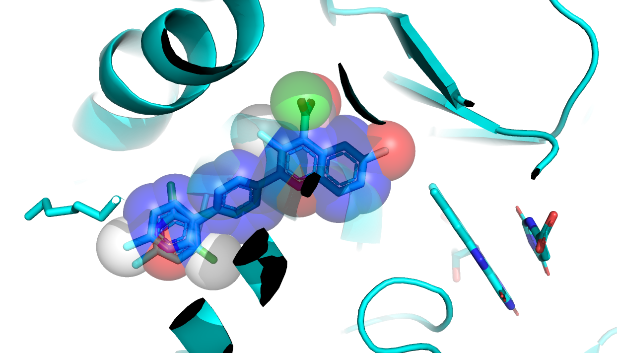
We have chosen the complex with PDB id 1D3G which is part of the DUD-E dataset as our target.
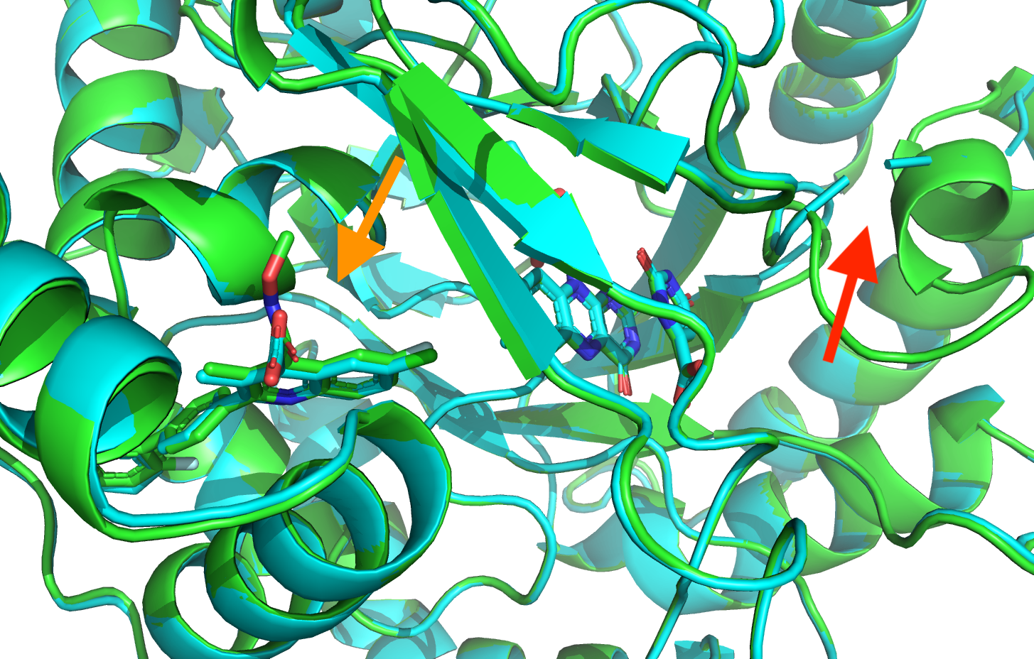
This is a complex of an inhibitory brequinar analong bound to the human dihydroorotate dehydrogenase receptor.
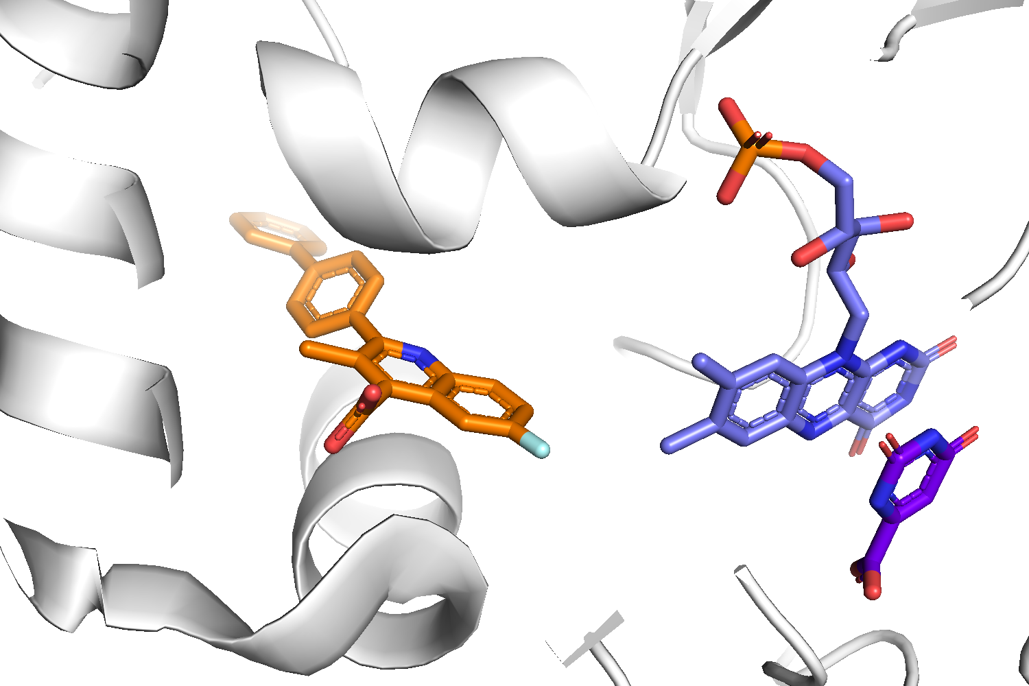
Binding site of the target complex (1D3G): The receptor is shown in white cartoon, whereas the brequinar analog (BRE) in orange sticks. The binding site also contains Orotate (ORO - purple sticks) and Flavin Mononucleotide (FMN - light blue sticks). BRE acts as an inhibitor of the oxidation of Dihydro-ORO -> ORO and the reduction of FMN -> dihydro-FMN.
Shape-restrained protocol outline
Briefly, the main steps of this protocol are the following:
- Identify and download potential templates of interest for our target of choice.
- Select one of the identified templates for the modelling of the complex.
- Prepare the input files for the docking.
- Perform the docking.
- Analyse and visualise the results.
Note: The shape-based protocol can be adapted into a pharmacophore-based protocol. Steps 2 and 3 can be adapted accordingly as described in the last section of this tutorial.
1. Identifying suitable templates
The nature of the binding site makes it clear that if we are to reproduce the chemical environment of the target complex
then the template we choose must also contain ORO and FMN in its binding site.
The first step requires we search one of the PDB portals (in our case we will make use of RCSB PDB portal) for
templates to extract the shape information we will use throughout the docking. After landing on the homepage of the
aforementioned RCSB portal we activate the advanced search functionality by clicking on the Advanced Search link
immediately below the search bar.
We will use the sequence of the receptor of our target complex as our primary search parameter. Clicking on the
‘Sequence’ tab of the advanced search parameters we are provided with two options to load the query sequence. Either
write/paste it manually using the large textbox or use a PDB id. We opt for the latter option. Writing 1D3G in the
PDB id box and clicking on the prompt loads the sequence in the larger textbox above. We also specify an Identity
Cutoff of 100% to make sure we limit the results to only relevant hits. Once this is done click on the search button
at the bottom on the right. In case a prompt window pops up simply click on ok.
Generating a tabular report using the “ligand” preset and saving it in .csv format allows us to gather all the data we
need to select a template for docking. The pre-generated file can be found in the provided data under data/ligands.csv.
Note that the file you create can differ from the pre-generated file provided as the PDB database is constantly updated.
A filtered version of it with only the required data can be found in the data/ligands_filtered.csv file.
To create the latter file we have filtered out the unnecessary ligands from the original file (ie the compounds common to all complexes such as ORO and FMN and also all crystallisation artifacts) and only kept the PDB id, ligand id and SMILES string for all
compounds.
2. Selecting the template
As is the case for any template-based modelling approach, the more similar the template is to the target complex the
higher the chance of a successful modelling outcome. In this protocol, we are emphasising ligand similarity over receptor
similarity, meaning we want the template and target compounds to be as similar as possible. The metric we have chosen as
our similarity measure is the Tversky coefficient (with alpha=0.2, and beta=0.8) computed over the Maximum Common Substructure (MCS) as calculated by the RDKit implementation.
This metric can be computed in a time-efficient manner and most importantly without prior knowledge of the structure
of the target compound and all that is required is the compound encoded in SMILES format (see data/target.smi and data/templates.smi).
The templates.smi file can be created from the following command:
grep -v SMILES data/ligands_filtered.csv | awk '{print $3,$1"_"$2}' > templates.smi
This file is provided at data/target.smi.
In general if the compound one is interested is part of a PDB structure then its SMILES
string can be found in the PDB database. Alternatively there are a plethora of computational chemistry
tools that can generate SMILES strings.
The next step involves computing the similarity values between our target (reference) compound and all template compounds
we identified through the RCSB search portal. For this we will use an RDKit-based implementation of the MCS procedure described
above. We provide a python-based implementation in the scripts/calc_mcs.py. Usage of the script is straightforward:
./scripts/calc_mcs.py -te templates.smi -ta data/target.smi | awk '{print $2}' > tmp
This command might takes a few seconds to complete. We choose to only keep the second column because we are only interested in the Tversky metric and the first column of the output is the Tanimoto metric. To create the similarities file:
These similarity values have also been precalculated and can be seen in the data/similarities.txt file.
The file is sorted according to the similarity value, meaning the compounds most similar to the target compound
are near the top of the file. From this point on, the selection of the most suitable template becomes a process of filtering out
the templates that are ill-suited for modelling (low quality, mutations near the binding site, missing density, etc.).
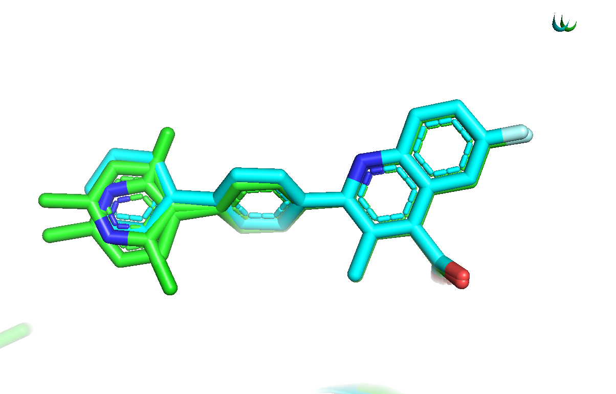
Two templates are highly similar, 2PRH and 7K2U with Tversky coefficients of 0.956 and 0.942, respectively.
A closer examination of the binding site of the most similar template, 2PRH, reveals missing density close to the ORO cofactor (segment 227-225).
Further 2PRH has a lower resolution (2.4Å) than that of 7K2U (1.72Å). For these reasons we select 7K2U for as template for the docking.
[Click here to see the comparison of 2PRH and 7K2U]
3. Preparing the input files for docking
3a. Preparing the receptor template and the shape PDB files
The docking-ready file created from entry 7K2U is available as data/template.pdb with all the crystallisation artifacts and double occupancies removed).
To achieve that we can use the following commands from pdb-tools; pdb_selaltloc and pdb_keepcoord.
The next step involves the creation of the shape (based on the template compound) that will be used for the docking. This
process requires the transformation of all heavy atoms of the template compound (named VU7) into shape beads.
The shape beads have all the same residue and atom names, namely SHA and their chainID for use in HADDOCK should be S.
Note that we used pdb_reres and pdb_reatom to renumber the shape starting at number 1.
At the same time we also need to remove the compound present in the template structure since that space is now occupied by the shape we just created.
grep -v VU7 data/template.pdb > template-final.pdb
3b. Generating an ensemble of conformations for the ligand to be docked
To make sure the tutorial we are presenting here sticks as closely as possible to a real-life modelling scenario we will be generating conformers starting from the SMILES string of the reference compound. For this, we will also use RDKit along with a predefined set of parameters that govern the behaviour of the program during the conformer generation.
The script we will use can be found in scripts/generate_conformers.py.
Running it with the -h flag will list all possible options the script
can be called with. We will run it with the optimal options that were estabilished during the benchmarking of this protocol benchmark.
./scripts/generate_conformers.py -i data/target.smi -p 3sr -c 50 -m -o conformers.pdb
The above command will create a conformers.pdb file in the current working directory.
We need to process the file to remove the redundant data in it and prepare it for docking.
grep -v CONECT conformers.pdb | sed -e 's/UNL/UNK/' | pdb_chain -B > t; mv t conformers.pdb
3c. Generating shape restraints for the ligand to be docked
We then need to create the restraints that will be used throughout the simulation to drive the generated compounds to the binding pocket. Since there are fewer atoms in the target compound than there are in the shape, we are defining the restraints from the target compound to the shape. For this, one distance restraint is defined from each ligand heavy atom to all shape atoms with an upper bound limit of 1Å.
In addition to the restraints that are meant to drive the compound to the binding pocket we also need to define restraints
between the cofactors and their coordinating residues to make sure they maintain their original geometry throughout the
simulation and don’t drift away in the flexible stage. This can be done with scripts/restrain_ligand.py:
And we concatenate the newly created restraint files into one with:
cat template-final_ORO.tbl template-final_FMN.tbl >cofactor_restraints.tbl
This concludes the preparation steps required for the receptor. However, we still need to prepare the compound structures
we will be using for docking. In order to make this tutorial as close as possible to a real-world application of this
protocol, instead of using a bound form of the compound (from this complex or a different one) we have pregenerated 3D
conformers with RDKit using only the compound SMILES. The conformer ensemble can be found in the data/conformers.pdb file.
4. Setting up the docking
For the docking we will use the new portal of HADDOCK2.4. If you are already
registered with HADDOCK or have been provided with course credential then you can proceed to job submission immediately.
Alternatively, you can request an account through the registration portal. Keep in mind that for this tutorial you will
have to request guru level access, this is done by selecting the Request Elevated Access in your user profile.
After logging in you are greeted with the first part of the submission portal. Make sure to use an informative name for the run.
-
Step1: Define a name for your docking run in the field “Job name”, e.g. shape-based-small-molecule.
-
Step2: Select the number of molecules to dock. Since this is a three-body docking between the template receptor, the template shape and the generated conformers so we should set the number of molecules to 3.
- Step3: Input the receptor protein PDB file. For this unfold the Molecule 1 - input if it isn’t already unfolded.
Molecule 1 - input -> PDB structure to submit -> Upload the file named template-final.pdb
Molecule 1 - input -> Fix molecule at its original position during it0? -> True
- Step4: Input the ensemble of ligand conformations PDB file. For this unfold the Molecule 2 - input if it isn’t already unfolded.
Molecule 2 - input -> PDB structure to submit -> Upload the file named conformers.pdb
Molecule 2 - input -> What kind of molecule are you docking? -> Ligand
- Step5: Input the shape PDB file. For this unfold the Molecule 3 - input if it isn’t already unfolded.
Molecule 3 - input -> PDB structure to submit -> Upload the file named shape.pdb
Molecule 3 - input -> Fix molecule at its original position during it0? -> True
Molecule 3 - input -> What kind of molecule are you docking? -> Shape
Molecule 3 - input -> Segment ID to use during the docking -> S
-
Step 6: Click on the “Next” button at the bottom left of the interface. This will upload the structures to the HADDOCK webserver where they will be processed and validated (checked for formatting errors). The server makes use of Molprobity to check side-chain conformations, eventually swap them (e.g. for asparagines) and define the protonation state of histidine residues.
-
Step 7: The second submission tab “Input Parameters” can be skipped entirely since we will be defining our restraints through tbl files instead of doing it through the interface. Click on “Next”.
-
Step 8: Define the distance restraints (both to the shape and to maintain the co-factors in place). For this unfold the Distance restraints menu if not already unfolded
For protein-ligand docking we advise to keep all hydrogen atoms (non-polar hydrogens are deleted by default by the server)
Distance restraints -> Remove non-polar hydrogens? -> False
Further we want to make use of all shape restraints. For this we should turn off the random removal of restraints (only affects the ambig restraints):
Distance restraints -> Randomly exclude a fraction of the ambiguous restraints (AIRs) -> False
- Step 9: Change the sampling parameters. For this unfold the Sampling parameters menu if not already unfolded
Since we have 16 conformations in the ligand ensembles, change the number of models to generate to 320 (20 per ligand conformation).
Sampling parameters -> Number of structures for rigid body docking -> 320
Sampling parameters -> Sample 180 degrees rotated solutions during rigid body EM -> False
For small molecule docking we do not recommend to perform the final refinement, but instead use the models from the semi-flexible refinement stage (it1).
Sampling parameters -> Perform final refinement? -> False
- Step 10: Change the interaction parameters. For this unfold the Energy and interaction parameter menu if not already unfolded
We scale down the interaction during rigid body docking (it0) to allow for better penetration of the ligand in possiblity buried binding sites.
- Step 10: Change the scoring function. For this unfold the Scoring parameter menu if not already unfolded
Because of the changes in Step 9 which can result in clashes, we should set the weight of the van der Waals energy term to 0 for it0
Scoring parameters -> Evdw 1 -> 0
- Step 11: Change the analysis parameters. For this unfold the Analysis parameter menu if not already unfolded
For this docking scenario we recommend to take the ranking of single structure and do not perform clustering.
Analysis parameters -> Full or limited analysis of results -> None
- Step 12: You are ready to dock! Click “Submit”. If everything went well your docking run has been added to the queue and might take anywhere from a few hours to a few days to finish depending on the load on our servers.
Note that prior to submission you also have the option to download the processed data (in the form of a tgz archive) and a .json file which contains all the settings and input structures for our run. We strongly recommend to download this file as it will allow you to repeat the run by using the file upload inteface of the HADDOCK webserver. This .json file can serve as input reference for the run, and could be provided as supplementary material in a publication. This file can also be edited to change a few parameters for example.
The generated json file for this shape-based submission is provided at data/job_params-shape.json.
Upon submission you will be presented with a web page which also contains a link to the previously mentioned .json file as well as some information about the status of the run.
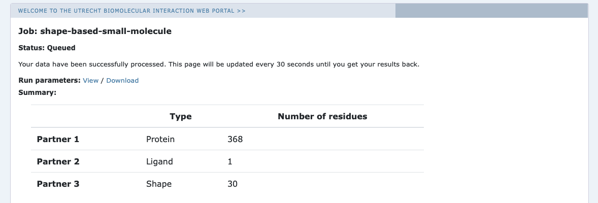
Currently your run should be queued but eventually its status will change to “Running” (the page is automatically refreshed):
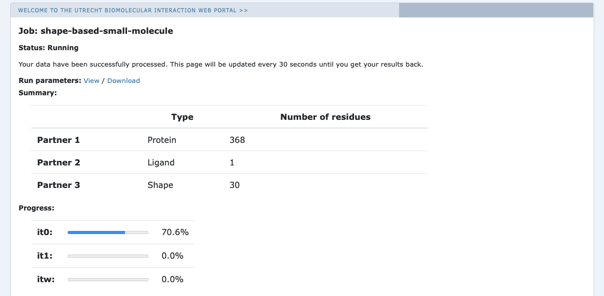
The page will give you a progress update of your and the results will appear upon completions (which can take between 1-2 hours to several hours (and even days) depending on the size of your system and the load of the server). You will be notified by e-mail once your job has successfully completed. This page can be closed, you can access your submitted runs via the Workspace page
5. Visualisation and analysis of results
Once your run has completed you will be presented with a result page showing the cluster statistics (in this case the statistics of the top10 single models) and some graphical representation of the data (and if not using course credentials, you will also be notified by e-mail).
5a - Inspecting the result page
While HADDOCK is running we can already start looking at precalculated results here (which have been derived using the exact same settings we used for our run). Just glancing at the page tells us that our run has been a success both in terms of the actual run and the post-processing that follows every run. Examining the summary page reveals that in total HADDOCK only clustered 10 models in 10 different clusters, effectively performing only single structure analysis. This was expected since we specified no analysis when setting up the run. Usually, clustering is a very helpful step when performing protein-protein docking with well-defined interfaces but we observed that it conveys no measurable benefit for this type of modelling (protein-small molecule) and therefore we skip it.
The bottom of the page gives you some graphical representations of the results, showing the distribution of the solutions for various measures (HADDOCK score, Van der Waals energy, etc.) as a function of the Fraction of Common Contact (FCC) and also with interface-RMSD from the best scoring model. The graphs are interactive and you can turn on and off specific clusters (single structures in this case), but also zoom in on specific areas of the plot.
A more consice way of looking at the breakdown of energetics per model is to look at the summary for each model which can be found immediately below the overall summary page. For example, for the top scoring model the HADDOCK score is -62.6 with a VdW, electrostatics, desolvation and Buried Surface Area (BSA) contribution of -42.1, -6.2, -6.6 and 771.1, respectively.
The HADDOCK score in this case corresponds to the it1 score (see for details the online manual pages). It is defined as:
HADDOCK-it1-score = 1.0 * Evdw + 1.0 * Eelec + 1.0 * Edesol + 0.1 * Eair - 0.01 * BSA
where Evdw is the intermolecular Van der Waals energy, Eelec the intermolecular electrostatic energy, Edesol represents an empirical desolvation energy term adapted from Fernandez-Recio et al. J. Mol. Biol. 2004, Eair the distance restraint energy and BSA the buried surface area in Å. The various components of the HADDOCK score are also reported for each cluster on the results web page.
5b - Visualisation of the models and comparison with the reference complex.
For a closer look at the top models we can use the link on results webpage just above the Cluster 1 line to download the top10 models, or simply click here.
Using the following command expand the contents of the tgz archive in your working directory:
tar xfz 76656-shape-based-small-molecule_summary.tgz
This will result in the creation of 10 PDB files in the current working directory. The files are named cluster*_1.pdb with
the values for * ranging between 1 and 10 reflecting the ranking of the top 10 models according to their haddock score,
with model cluster1_1.pdb being the model with the overall best HADDOCK score.
Important: Please note that the cluster number is not its ranking but a measure of how populated it is. Cluster 1 will always contain the most models, but it might not be the top ranking cluster. The order on the results webpage corresponds to the ranking. Please check the HADDOCK Manual for more information.
With the following command we can load the top 10 models into PyMOL (sorted by HADDOCK score) along with the reference compound provided in the data directory for
closer examination.
pymol data/1d3g.pdb cluster[1-9]_1.pdb cluster10_1.pdb
After PyMOL has finished loading, we can remove all artifacts and superimpose all models on the reference compound with the following PYMOL commands:
remove resn hoh+so4+act+ddq
alignto 1d3g and chain A
zoom
And the following PyMOL commands allow us to get a better overview of the binding site:
remove hydro
hide everything, resn sha
util.cbc
color white, 1d3g
util.cnc
zoom resn UNK
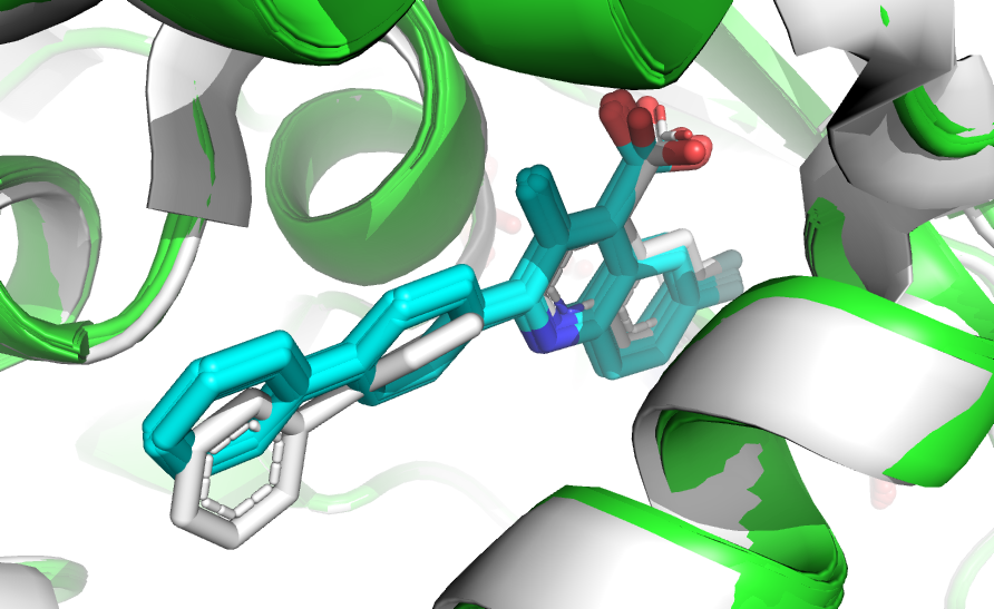
The top 10 models have very similar HADDOCK scores (you need to download full run to access these values), and a visual analysis reveals that they also adopt similar binding modes and are very close to the reference structure.
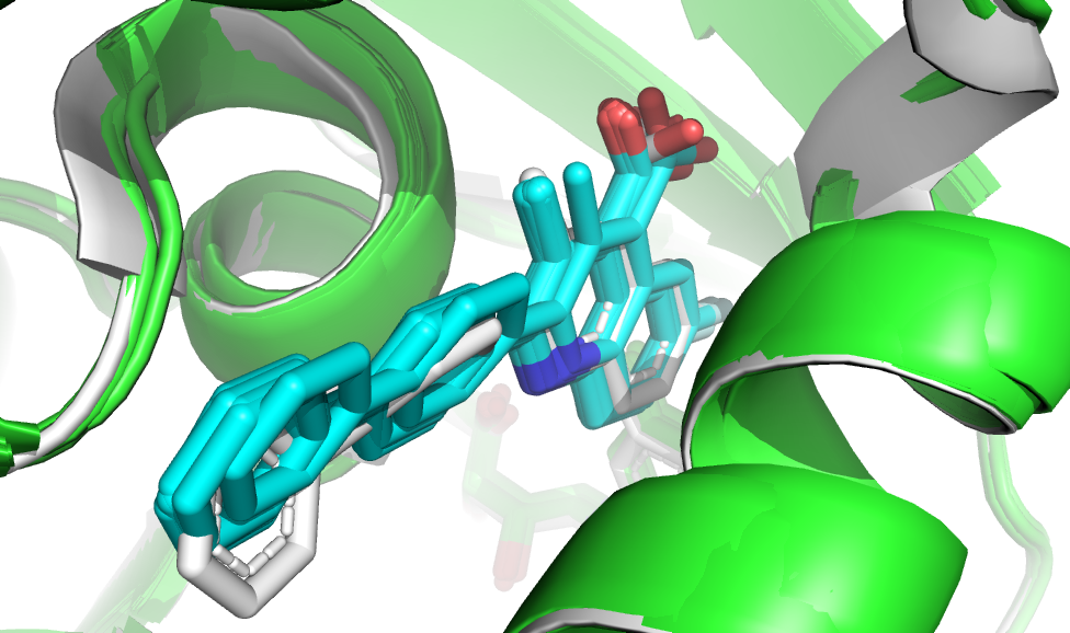
Superimposition of the top10 scoring pose onto the reference complex (in white).
As part of the analysis we can also compute the symmetry-corrected ligand RMSD for our model of choice. Before doing that we should make sure the models are aligned to the target. This can be done using for example the ProFit software.
If ProFit is installed in your system you can use the provided scripts/izone to align a model to the target on the protein interface residues. The script will write the aligned file as tmp.pdb. For the top-scoring compound the commands to use are:
obrms (installed with Anaconda) reports a ligand RMSD value of 0.74 indicating excellent agreement between model and reference structures.
If you don’t have ProFit installed you can use instead PyMOL to fit the models on the binding site residues: Assuming you still have PyMOL open and have performed the above commands, do the following to fit the top model (cluster1) onto the binding site of the target:
Then save the aligned cluster1_1 by selecting from the PyMOL menu:
File -> Export molecule… Selection -> cluster1_1 Click on Save… Select as ouptut format PDB (*.pdb *.pdb.gz) Name your file tmp.pdb, note its location and move it to your working directory
You can then calculate the ligand RMSD with:
If we want to examine the run in greater detail then we can download the archive of the entire run from here. After extraction, this will create the 76481-shape-based-small-molecule directory in
the current working directory. The final models can be found under the structures/it1 subdirectory. There are 200
PDB files in total and their ranking along with their scores can be seen in the file.list file.
The above command should show the same HADDOCK scores as what we already saw for the top 10 models.
Pharmacophore-based protocol
The shape-based protocol described above can be adapted into a pharmacophore-based protocol in which the beads used to drive the docking are assigned pharmacophore properties.
This protocol requires modifications of the aforedescribed Steps 2 and 4.
2.pharm - Template selection
In this protocol, we want template molecules to be as similar as possible as the target ligand in terms of pharmacophore properties. The metric we have chosen is to measure this similarity is the Tanimoto coefficient (Tc) computed over the 2D pharmacophore fingerprints as computed with RDKIT.
To ensure correct 2D pharmacophore descriptor computation, we need to use SDF files as input files.
The provided data/templates.smi file can be created from the following command:
grep -v SMILES data/ligands_filtered.csv | awk '{print $3,$1"_"$2}' > templates.smi
The target.smi file we create manually by copying and pasting the SMILES string from its PDB RCSB page.
Both files are available from the data directory.
SMILES can be converted into SDF files (if you want to use the files you just created, remove ./data/ from the commands below):
The generated templates.sdf file contains multiple molecules. It must be split in a way to have one file per molecule.
The next step involves computing the similarity values between our target (reference) compound and all template compounds we have identified through the RCSB search portal.
For this we will use an RDKit-based implementation of the 2D pharmacophore fingerprints computation.
We provide a python-based implementation in the script pharm2D_Tc.py. Usage of the script is straightforward:
python ./scripts/pharm2D_Tc.py target/ templates/
The script will return a file entitled sim.Tc containing all Tc values. The line flagged with best highlights the most similar template.
These similarity values have also been precalculated and can be seen in the sim.Tc file in the data directory.
A closer examination of the binding site of template 6CJF (provided in the data directory) reveals that the 2-chloro-6-methylpyridin group
of the F54 ligand may adopt two distinct conformations. A thorough examination of the 6CJF PDB file shows that the conformation A is associated
to an occupancy factor of 0.66 against 0.34 for the conformation B.
Since the conformation A is more populated than conformation B, we will select it as our template of interest and renumber the atom starting from 1 (required for the pharmacophore features generation - see below).
[Click here to see binding site details]
3.pharm - Preparing the input files for docking
3a.pharm - Preparing the receptor template and the pharmacophore shape
The docking-ready receptor file is available as data/template_pharm.pdb (with all the crystallisation artifacts and double occupancies removed).
To achieve that we can use the following command making use of the pdb_selaltloc and pdb_keepcoord utilities which are
part of the pdb-tools package.
TO ADD COMMAND
The next step involves the creation of the pharmacophore shape (based on the template compound) that will be used for the docking. This process requires the addition of pharmacophore information into the PDB file and transformation of all heavy atoms of the template compound into pharmacophore beads.
The pharmacophore information is encoded in the occupancy factor column of the PDB file with different values corresponding to different pharmacophores:
- 0.10 ➞ Donor
- 0.20 ➞ Acceptor
- 0.30 ➞ NegIonizable
- 0.40 ➞ PosIonizable0
- 0.50 ➞ ZnBinder
- 0.60 ➞ Aromatic
- 0.70 ➞ Hydrophobe
- 0.80 ➞ LumpedHydrophobe
Warning make sure that the atomic numbers of F54.pdb start at number 1. The provided data/F54.pdb has been renumbered (this was done using pdb_reatom).
The pharmacophore features can be added to the template ligand with scripts/add_atom_features.py.
This is an essential step to create the pharmacophore shape. Here again, it is important to deduce pharmacophore features from a SDF file, which is better handled by RDKIT than PDB files.
In order to have the same atom ordering in the SDF file and the PDB file to which features will be assigned, you can use openbabel to convert the PDB file into an SDF file.
obabel -ipdb F54.pdb -osdf -O F54.sdf
python ./scripts/add_atom_features.py F54.sdf F54.pdb
The created F54_features.pdb file contains pharmacophore information in the occupancy factor column (a reference file is provided in the data directory).
The template ligand can now be converted into a shape (shape_pharm.pdb) with the following script:
python ./scripts/lig2shape.py pharm F54_features.pdb > shape_pharm.pdb
At the same time we also need to remove the compound present in the template structure since that space is now occupied by the shape we just created.
grep -v F54 data/template_pharm.pdb > template-final_pharm.pdb
Pharmacophore shape used to guide the docking.
3b.pharm - Generating target ligand conformers and encoding the pharmacophore information
In order to account for the ligand flexibility during the docking, we will provide several conformations of the target ligand. We will use the conformers used in the shape based protocol and we will add pharmacophore features using the following commands:
3c.pharm - Generating the pharmacophore shape restraints
We then need to create the distance restraints that will be used throughout the docking to drive the generated compounds to the binding pocket. The pharmacophore restraints are defined from the target to the pharmacophore shape:
For example the following distance restraint:
assi (segid B and name C2) (segid S and (attr q == 0.60) ) 1.0 1.0 0.0
will restrain the C2 atom of the ligand with segid B to be at proximity (within 1Å) of an Aromatic bead of the shape.
Provided that you generated 3D conformers for your target ligand, stored them in a file called conformers.pdb, and added the pharmacophore features information (with the add_atom_features.py script), you can generate the pharmacophore restraints to guide the docking. As mentioned earlier, this file is provided in this tutorial for convenience (conformers were generated with RDKIT).
./scripts/generate_restraints_from_target.py data/conformers.pdb
This command will create a distance restraints file named shape_pharm_restraints.tbl (also available in the data directory).
In addition to the restraints that are meant to drive the compound to the binding pocket we also need to define restraints
between the cofactors and their coordinating residues to make sure they maintain their original geometry throughout the
simulation and don’t drift away in the flexible stage. This can be done using scripts/restrain_ligand.py:
And we concatenate the newly created restraint files into one with:
cat template-final_pharm_ORO.tbl template-final_pharm_FMN.tbl >cofactor_restraints_pharm.tbl
The pre-calculated restraints are provided at data/cofactor_restraints_pharm.tbl.
4.pharm - Setting up the pharmacophore-based docking
The docking preparation is detailed in the docking description from the shape-based protocol. From the described steps you only need to adapt the following steps keeping all other steps similar:
- Step3: Input the receptor protein PDB file selecting the selected template
Molecule 1 - input -> PDB structure to submit -> Upload the file named template-final_pharm.pdb
- Step5: Input the shape PDB file selected the proper shape for the pharma procotol.
Molecule 3 - input -> PDB structure to submit -> Upload the file named shape_pharm.pdb
- Step 8: Define the distance restraints (both to the shape and to maintain the co-factors in place).
Make sure to change all other required parameters as previously explained and submit your run.
As reference the .json file generate for this tutorial is available under data/job_params-pharm.json
5.pharm Visualisation and analysis of results
While HADDOCK is running we can already start looking at precalculated results (which have been derived using the exact same settings we used for our run). The precalculated run can be found here. Just glancing at the page tells us that our run has been a success both in terms of the actual run and the post-processing that follows every run. Examining the summary page reveals that in total HADDOCK only clustered 10 models in 10 different clusters, effectively performing only single structure analysis. This was expected since we specified no analysis when setting up the run. Usually, clustering is a very helpful step when performing protein-protein docking with well-defined interfaces but we find that it conveys no measurable benefit for this type of modelling (protein-small molecule) and therefore we skip it.
For a closer look at the top models we can use the link on results webpage just above the Cluster 1 line to download the top10 models, or simply click here.
Using the following command expand the contents of the .tgz archive in your working directory:
tar xfz 76693-pharm-based-small-molecule_summary.tgz
This will result in the creation of 10 PDB files in the current working directory. The files are named cluster*_1.pdb with
the values for * ranging between 1 and 10 reflecting the ranking of the top 10 models according to their haddock score,
with model cluster1_1.pdb being the model with the overall best HADDOCK score.
Important: plase note that the cluster number is not its ranking but a measure of how populated it is. Cluster 1 will always contain the most models, but it might not be the top ranking cluster. The order on the results webpage corresponds to the ranking. Please check the HADDOCK Manual for more information.
With the following command we can load the top 10 models into PyMOL (sorted by HADDOCK score) along with the reference compound provided in the data directory for
closer examination.
pymol data/1d3g.pdb cluster[1-9]_1.pdb cluster10_1.pdb
After PyMOL has finished loading, we can remove all artifacts and superimpose all models on the reference compound with the following PyMOL commands:
remove resn hoh+so4+act+ddq
alignto 1d3g and chain A
zoom
And the following PyMOL commands allow us to get a better overview of the binding site:
remove hydro
hide everything, resn sha
util.cbc
color white, 1d3g
util.cnc
zoom resn UNK
The visual analysis reveals that the top 10 models not only have very similar HADDOCK scores but they also adopt similar binding modes and are very close to the reference structure.
Superimposition of the top10 scoring pose onto the reference complex (in white).
As part of the analysis we can also compute the symmetry-corrected ligand RMSD for our model of choice. Before doing that we should make sure the models are aligned to the target. This can be done using for example the ProFit software.
If installed in your system you can use the provided data/izone ProFit script to align a model to the target on the protein interface residues. The script will write the aligned file as tmp.pdb. For the top-scoring compound the commands to use are:
obrms reports a ligand RMSD value of 1.09Å indicating again excellent agreement between model and reference structures for this adaptation of the shape-restrained docking protocol.
If you don’t have ProFit installed you can use instead PyMOL to fit the models on the binding site residues: Assuming you still have PyMOL open and have performed the above commands, do the following to fit the top model (cluster1) onto the binding site of the target:
Then save the aligned cluster1_1 by selecting from the PyMOL menu:
File -> Export molecule… Selection -> cluster1_1 Click on Save… Select as ouptut format PDB (*.pdb *.pdb.gz) Name your file tmp.pdb, note its location and move it to your working directory
You can then calculate the ligand RMSD with:
If we want to examine the run in greater detail then we can download the archive of the entire run from [here]
(https://wenmr.science.uu.nl/haddock2.4/run/4242424242/76693-pharm-based-small-molecule.tgz){:target=”_blank”}
and expand it using the same command as above. This will create the 76693-pharm-based-small-molecule directory in
the current working directory. The final models can be found under the structures/it1 subdirectory. There are 200
PDB files in total and their ranking along with their scores can be seen in the file.list file.
The above command should show the same HADDOCK scores as what we already saw for the top 10 models.
Congratulations!
You have completed this tutorial. If you have any questions or suggestions, feel free to contact us via e-mail or asking a question through our support center.
And check also our education web page where you will find more tutorials!