Low-sampling antibody-antigen modelling tutorial using a local version of HADDOCK3

This tutorial consists of the following sections:

Introduction
Setup/Requirements
HADDOCK general concepts
A brief introduction to HADDOCK3
Software requirements
Preparing PDB files for docking
Defining restraints for docking
Setting up the docking with HADDOCK3
- HADDOCK3 execution modes
- Docking Scenario: Paratope - NMR-epitope
Analysis of docking results
Visualization of the models
BONUS: Does the antibody bind to a known interface of interleukin? ARCTIC-3D analysis
BONUS: Alphafold2 for antibody-antigen complex structure prediction
Conclusions
Congratulations! 🎉

Introduction

This tutorial demonstrates the use of the new modular HADDOCK3 version for predicting the structure of an antibody-antigen complex using knowledge of the hypervariable loops on the antibody (i.e., the most basic knowledge) and epitope information identified from NMR experiments for the antigen to guide the docking.

An antibody is a large protein that generally works by attaching itself to an antigen, which is a unique site of the pathogen. The binding harnesses the immune system to directly attack and destroy the pathogen. Antibodies can be highly specific while showing low immunogenicity, which is achieved by their unique structure. The fragment crystallizable region (Fc region) activates the immune response and is species-specific, i.e. the human Fc region should not induce an immune response in humans. The fragment antigen-binding region (Fab region) needs to be highly variable to be able to bind to antigens of various nature (high specificity). In this tutorial we will concentrate on the terminal variable domain (Fv) of the Fab region.

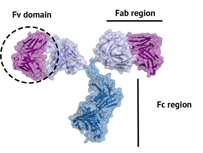
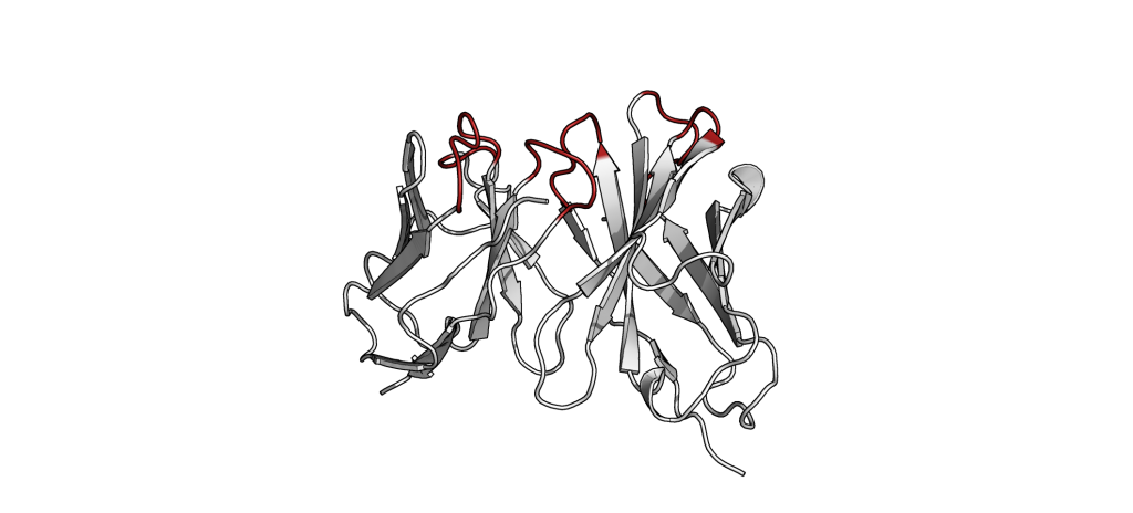
The small part of the Fab region that binds the antigen is called paratope. The part of the antigen that binds to an antibody is called epitope. The paratope consists of six highly flexible loops, known as complementarity-determining regions (CDRs) or hypervariable loops whose sequence and conformation are altered to bind to different antigens. CDRs are shown in red in the figure below:

In this tutorial we will be working with Interleukin-1β (IL-1β) (PDB code 4I1B) as an antigen and its highly specific monoclonal antibody gevokizumab (PDB code 4G6K) (PDB code of the complex 4G6M).

Throughout the tutorial, colored text will be used to refer to questions or instructions, and/or PyMOL commands.

This is a question prompt: try answering it! This an instruction prompt: follow it! This is a PyMOL prompt: write this in the PyMOL command line prompt! This is a Linux prompt: insert the commands in the terminal!

Setup/Requirements

In order to follow this tutorial you will need to work on a Linux or MacOSX system. We will also make use of PyMOL (freely available for most operating systems) in order to visualize the input and output data.

Further we are providing pre-processed PDB files for docking and analysis (but the preprocessing of those files will also be explained in this tutorial). The files have been processed to facilitate their use in HADDOCK and for allowing comparison with the known reference structure of the complex.

For this, navigate through the terminal to the tutorial directory:

cd /home/utente/BioExcel_SS_2023/HADDOCK

In it you should find the following directories and files:

haddock3: Contains the HADDOCK3 source code with some usage examples
pdbs: Contains the pre-processed PDB files
restraints: Contains the interface information and the corresponding restraint files for HADDOCK
runs: Contains pre-calculated run results for the various protocols in this tutorial
scripts: Contains a variety of scripts used in this tutorial
docking-antibody-antigen-CDR-NMR-CSP*.cfg: the different HADDOCK3 configuration files that can be used in the tutorial

If you are working from your own computer you download this zip archive. Remember that on your local machine you’ll have to install CNS and HADDOCK3.

HADDOCK general concepts

HADDOCK (see https://www.bonvinlab.org/software/haddock2.4) is a collection of python scripts derived from ARIA (https://aria.pasteur.fr) that harness the power of CNS (Crystallography and NMR System – https://cns-online.org) for structure calculation of molecular complexes. What distinguishes HADDOCK from other docking software is its ability, inherited from CNS, to incorporate experimental data as restraints and use these to guide the docking process alongside traditional energetics and shape complementarity. Moreover, the intimate coupling with CNS endows HADDOCK with the ability to actually produce models of sufficient quality to be archived in the Protein Data Bank.

A central aspect to HADDOCK is the definition of Ambiguous Interaction Restraints or AIRs. These allow the translation of raw data such as NMR chemical shift perturbation or mutagenesis experiments into distance restraints that are incorporated in the energy function used in the calculations. AIRs are defined through a list of residues that fall under two categories: active and passive. Generally, active residues are those of central importance for the interaction, such as residues whose knockouts abolish the interaction or those where the chemical shift perturbation is higher. Throughout the simulation, these active residues are restrained to be part of the interface, if possible, otherwise incurring in a scoring penalty. Passive residues are those that contribute for the interaction, but are deemed of less importance. If such a residue does not belong in the interface there is no scoring penalty. Hence, a careful selection of which residues are active and which are passive is critical for the success of the docking.

A brief introduction to HADDOCK3

HADDOCK3 is the next generation integrative modelling software in the long-lasting HADDOCK project. It represents a complete rethinking and rewriting of the HADDOCK2.X series, implementing a new way to interact with HADDOCK and offering new features to users who can now define custom workflows.

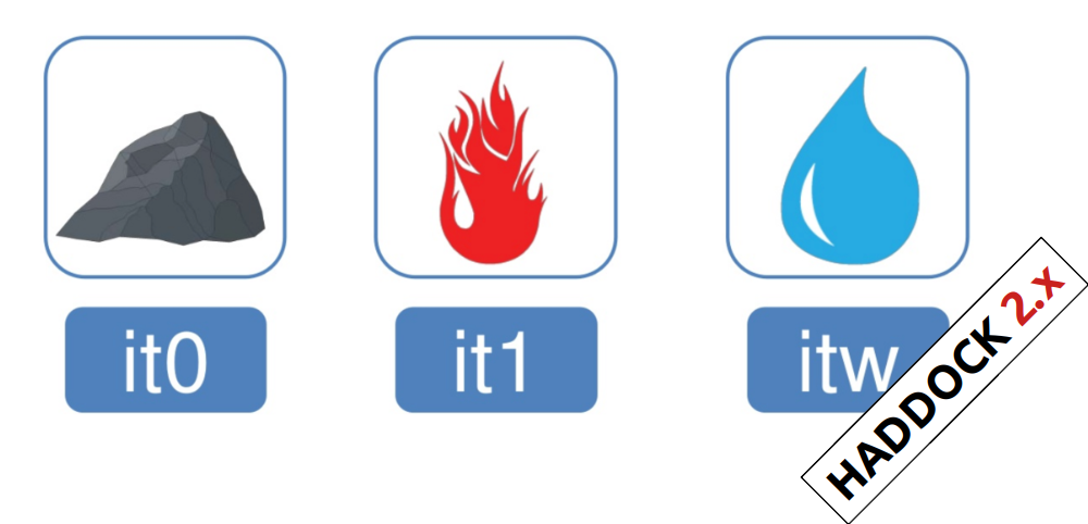
In the previous HADDOCK2.x versions, users had access to a highly parameterisable yet rigid simulation pipeline composed of three steps: rigid-body docking (it0), semi-flexible refinement (it1), and final refinement (itw).

In HADDOCK3, users have the freedom to configure docking workflows into functional pipelines by combining the different HADDOCK3 modules, thus adapting the workflows to their projects. HADDOCK3 has therefore developed to truthfully work like a puzzle of many pieces (simulation modules) that users can combine freely. To this end, the “old” HADDOCK machinery has been modularized, and several new modules added, including third-party software additions. As a result, the modularization achieved in HADDOCK3 allows users to duplicate steps within one workflow (e.g., to repeat twice the it1 stage of the HADDOCK2.x rigid workflow).

Note that, for simplification purposes, at this time, not all functionalities of HADDOCK2.x have been ported to HADDOCK3, which does not (yet) support NMR RDC, PCS and diffusion anisotropy restraints, cryo-EM restraints and coarse-graining. Any type of information that can be converted into ambiguous interaction restraints can, however, be used in HADDOCK3, which also supports the ab initio docking modes of HADDOCK.

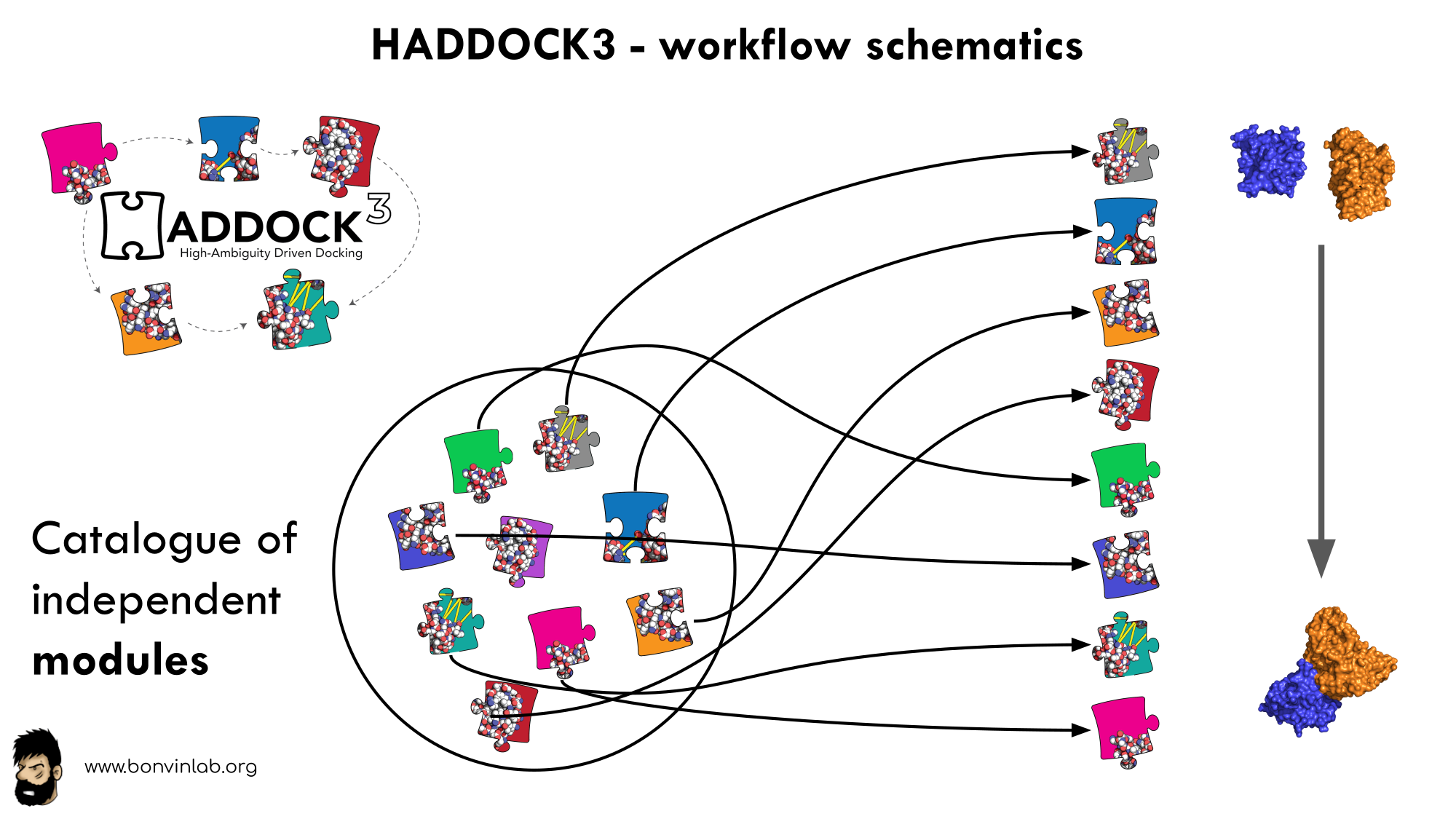
To keep HADDOCK3 modules organized, we catalogued them into several categories. But, there are no constraints on piping modules of different categories.

The main module categories are “topology”, “sampling”, “refinement”, “scoring”, and “analysis”. There is no limit to how many modules can belong to a category. Modules are added as developed, and new categories will be created if/when needed. You can access the HADDOCK3 documentation page for the list of all categories and modules. Below is a summary of the available modules:

Topology modules
- topoaa: generates the all-atom topologies for the CNS engine.
Sampling modules
- rigidbody: Rigid body energy minimization with CNS (it0 in haddock2.x).
- lightdock: Third-party glow-worm swam optimization docking software.
Model refinement modules
- flexref: Semi-flexible refinement using a simulated annealing protocol through molecular dynamics simulations in torsion angle space (it1 in haddock2.x).
- emref: Refinement by energy minimisation (itw EM only in haddock2.4).
- mdref: Refinement by a short molecular dynamics simulation in explicit solvent (itw in haddock2.X).
Scoring modules
- emscoring: scoring of a complex performing a short EM (builds the topology and all missing atoms).
- mdscoring: scoring of a complex performing a short MD in explicit solvent + EM (builds the topology and all missing atoms).
Analysis modules
- caprieval: Calculates CAPRI metrics (i-RMSD, l-RMSD, Fnat, DockQ) with respect to the top scoring model or reference structure if provided.
- clustfcc: Clusters models based on the fraction of common contacts (FCC)
- clustrmsd: Clusters models based on pairwise RMSD matrix calculated with the rmsdmatrix module.
- rmsdmatrix: Calculates the pairwise RMSD matrix between all the models generated in the previous step.
- seletop: Selects the top N models from the previous step.
- seletopclusts: Selects top N clusters from the previous step.

The HADDOCK3 workflows are defined in simple configuration text files, similar to the TOML format but with extra features. Contrarily to HADDOCK2.X which follows a rigid (yet highly parameterisable) procedure, in HADDOCK3, you can create your own simulation workflows by combining a multitude of independent modules that perform specialized tasks.

Software requirements

Installing CNS

The other required piece of software to run HADDOCK is its computational engine, CNS (Crystallography and NMR System – https://cns-online.org). CNS is freely available for non-profit organizations. In order to get access to all features of HADDOCK you will need to compile CNS using the additional files provided in the HADDOCK distribution in the varia/cns1.3 directory. Compilation of CNS might be non-trivial. Some guidance on installing CNS is provided in the online HADDOCK3 documentation page here.

In this tutorial CNS has already been installed at /usr/local/cns_solve_1.3/, so you don’t have to worry.

Installing HADDOCK3

In this tutorial we will make use of the HADDOCK3 version. HADDOCK3 is already pre-installed in your system.

To make sure the HADDOCK3 is properly installed activate its conda environment:

conda activate haddock3

and then type

haddock3 -h

in the terminal. You should see a small help message explaining how to use the software.

In case you want to obtain HADDOCK3 for another platform, navigate to its repository, fill the registration form, and then follow the installation instructions.

Auxiliary software

PDB-tools: A useful collection of Python scripts for the manipulation (renumbering, changing chain and segIDs…) of PDB files is freely available from our GitHub repository. pdb-tools is automatically installed with HADDOCK3. If you have activated the HADDOCK3 Python environment you have access to the pdb-tools package.

PyMol: We will make use of PyMol for visualization. If not already installed on your system, download and install PyMol.

Preparing PDB files for docking

In this section we will prepare the PDB files of the antibody and antigen for docking. Crystal structures of both the antibody and the antigen in their free forms are available from the PDBe database. In the case of the antibody which consists of two chains (L+H) we will have to prepare it for use in HADDOCK such as it can be treated as a single chain with non-overlapping residue numbering. For this we will be making use of pdb-tools from the command line.

Note that pdb-tools is also available as a web service.

Note: Before starting to work on the tutorial, make sure to activate haddock3

conda activate haddock3

Preparing the antibody structure

Using PDB-tools we will download the unbound structure of the antibody from the PDB database (the PDB ID is 4G6K) and then process it to have a unique chain ID (A) and non-overlapping residue numbering by renumbering the merged pdb (starting from 1).

This can be done from the command line with:

The first command fetches the PDB ID, selects the heavy chain (H) and removes water and heteroatoms (in this case no co-factor is present that should be kept). An important part for antibodies is the pdb_fixinsert command that fixes the residue numbering of the HV loops: Antibodies often follow the Chothia numbering scheme and insertions created by this numbering scheme (e.g. 82A, 82B, 82C) cannot be processed by HADDOCK directly. As such renumbering is necessary before starting the docking. Then, the command pdb_selres selects only the residues from 1 to 120, so as to consider only the variable domain (FV) of the antibody. This allows to save a substantial amount of computational resources.

The second command does the same for the light chain (L) with the difference that the light chain is slightly shorter and we can focus on the first 107 residues.

The third and last command merges the two processed chains and assign them unique chain and segIDs, resulting in the HADDOCK-ready 4G6K_clean.pdb file. You can view its sequence running:

pdb_tofasta 4G6K_clean.pdb

Note that the corresponding files can be found in the pdbs directory of the archive you downloaded.

Machine-learning-based modelling of antibodies

The release of Alphafold2 in late 2020 has brought structure prediction methods to a new frontier, providing accurate models for the majority of known proteins. This revolution did not spare antibodies, with Alphafold2-multimer and other prediction methods (most notably ABodyBuilder2, from the ImmuneBuilder suite) performing nicely on the variable regions.

For a short introduction to AI and AlphaFold refer to this other tutorial introduction.

CDR loops are clearly the most challenging region to be predicted given their high sequence variability and flexibility. Multiple Sequence Alignment (MSA)-derived information is also less useful in this context.

Here we will see whether the antibody models given by Alphafold2-multimer and ABodyBuilder2 can be used to target the antigen in place of the standard unbound form, which is not usually available.

We already ran the prediction with these two tools, and you can find them in the pdbs directory (with names 4g6k_Abodybuilder2.pdb and 4g6k_AF2_multimer.pdb).

Let’s preprocess these models!

Now the Alphafold2-multimer top ranked structure. By default it is written to disk with chains A and B.

Let’s load the three cleaned antibody structures in Pymol to see whether they resemble the experimental unbound structure.

File menu -> Open -> select 4G6K_clean.pdb File menu -> Open -> select 4G6K_abb_clean.pdb File menu -> Open -> select 4G6K_af2_clean.pdb

We now use the backbone RMSD to align the machine learning models to the experimental structure. alignto 4G6K_clean

Which structure (between 4G6K_abb_clean.pdb and 4G6K_af2_clean.pdb) is closer to the unbound conformation?

Both ABodyBuilder2 and Alphafold2 can give an ensemble of models in output. All the structures in these ensembles may be used as input antibody molecules in HADDOCK.

The remaining of the tutorial will consider only the experimental unbound structure, but you can use your preprocessed predicted structures simply by substituting 4G6K_clean.pdb with either 4G6K_abb_clean.pdb or 4G6K_af2_clean.pdb.

Preparing the antigen structure

Using PDB-tools we will download the structure from the PDB database (the PDB ID is 4I1B), remove the hetero atoms and then process it to assign it chainID B.

Defining restraints for docking

Before setting up the docking we need first to generate distance restraint files in a format suitable for HADDOCK. HADDOCK uses CNS as computational engine. A description of the format for the various restraint types supported by HADDOCK can be found in our Nature Protocol paper, Box 4.

Distance restraints are defined as:

assign (selection1) (selection2) distance, lower-bound correction, upper-bound correction

The lower limit for the distance is calculated as: distance minus lower-bound correction and the upper limit as: distance plus upper-bound correction. The syntax for the selections can combine information about chainID - segid keyword -, residue number - resid keyword -, atom name - name keyword. Other keywords can be used in various combinations of OR and AND statements. Please refer for that to the online CNS manual.

We will shortly explain in this section how to generate both ambiguous interaction restraints (AIRs) and specific distance restraints for use in HADDOCK illustrating a scenario in which no a priori knowledge is available about the antibody binding site, but in which the antigen epitope has been pinpointed by an NMR chemical shift perturbation experiment.

Information about various types of distance restraints in HADDOCK can also be found in our online manual pages.

Identifying the paratope of the antibody

Nowadays there are several computational tools that can identify the paratope (the residues of the hypervariable loops involved in binding) from the provided antibody sequence. In this tutorial we are providing you the corresponding list of residue obtained using ProABC-2. ProABC-2 uses a convolutional neural network to identify not only residues which are located in the paratope region but also the nature of interactions they are most likely involved in (hydrophobic or hydrophilic). The work is described in Ambrosetti, et al Bioinformatics, 2020.

The corresponding paratope residues (those with either an overall probability >= 0.4 or a probability for hydrophobic or hydrophilic > 0.3) are:

31,32,33,34,35,52,54,55,56,100,101,102,103,104,105,106,151,152,169,170,173,211,212,213,214,216

The numbering corresponds to the numbering of the 4G6K_clean.pdb PDB file.

Let us visualize those onto the 3D structure. For this start PyMOL and load 4G6K_clean.pdb

File menu -> Open -> select 4G6K_clean.pdb

We will now highlight the predicted paratope. In PyMOL type the following commands:

color white, all select paratope, (resi 31+32+33+34+35+52+54+55+56+100+101+102+103+104+105+106+151+152+169+170+173+211+212+213+214+216)
color red, paratope

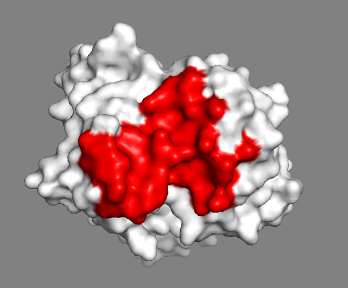
Can you identify the H3 loop? H stands for heavy chain (the first domain in our case with lower residue numbering). H3 is typically the longest loop.

Let us now switch to a surface representation to inspect the predicted binding site.

color white, all show surface
color red, paratope

Inspect the surface.

Do the identified residues form a well defined patch on the surface?

See surface view of the paratope

Antigen: NMR-mapped epitope information

The article describing the crystal structure of the antibody-antigen complex we are modelling also reports on experimental NMR chemical shift titration experiments to map the binding site of the antibody (gevokizumab) on Interleukin-1β. The residues affected by binding are listed in Table 5 of Blech et al. JMB 2013:

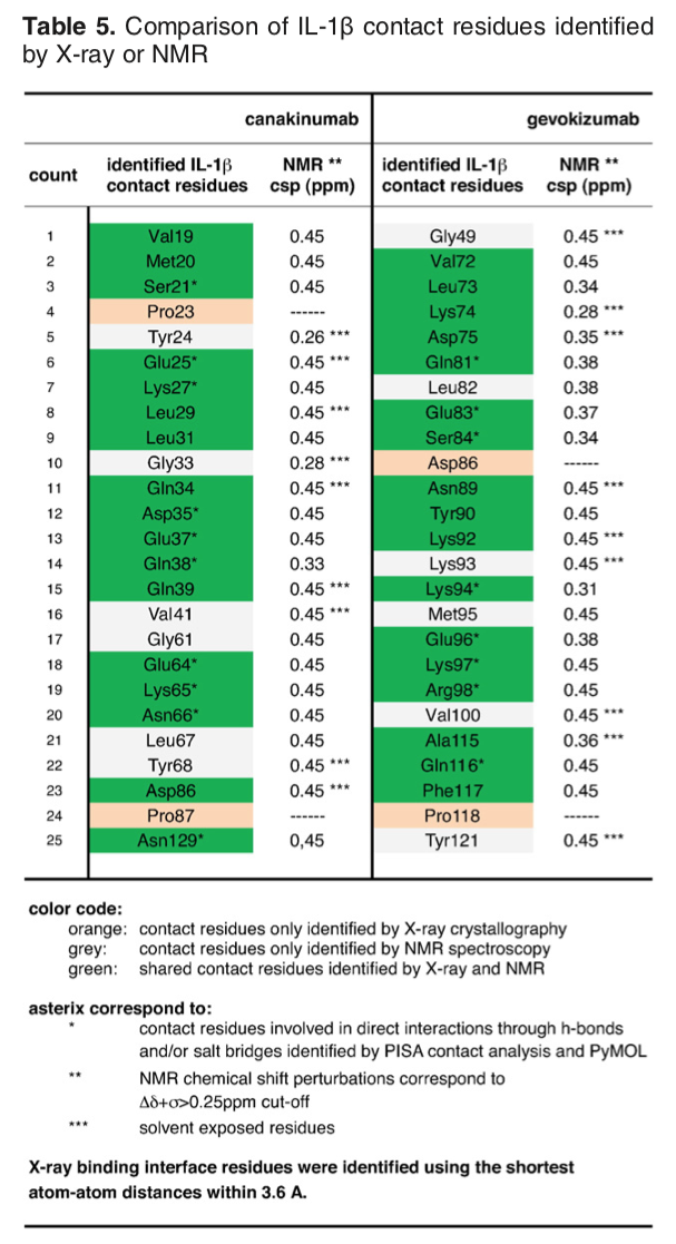
The list of binding site (epitope) residues identified by NMR is:

72,73,74,75,81,83,84,89,90,92,94,96,97,98,115,116,117

We will now visualize the epitope on Interleukin-1β. For this start PyMOL and from the PyMOL File menu open the provided PDB file of the antigen.

File menu -> Open -> select 4I1B_clean.pdb

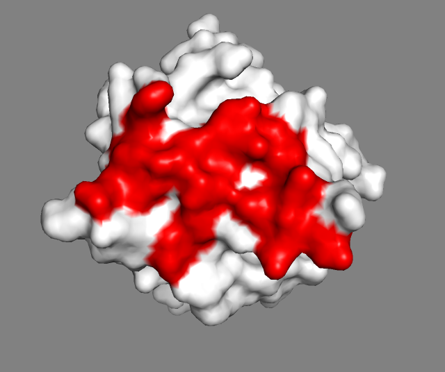
color white, all show surface select epitope, (resi 72+73+74+75+81+83+84+89+90+92+94+96+97+98+115+116+117) color red, epitope

Inspect the surface.

Do the identified residues form a well defined patch on the surface?

The answer to that question should be yes, but we can see some residues not colored that might also be involved in the binding - there are some white spots around/in the red surface.

See surface view of the epitope identified by NMR

In HADDOCK we are dealing with potentially incomplete binding sites by defining surface neighbors as passive residues. These are added to the definition of the interface but will not lead to any energetic penalty if they are not part of the binding site in the final models, while the residues defined as active (typically the identified or predicted binding site residues) will. When using the HADDOCK server, passive residues will be automatically defined. Here since we are using a local version, we need to define those manually.

This can easily be done using a script from our haddock-tools repository, which is also provided for convenience in the scripts directly of the archive you downloaded for this tutorial:

python ./scripts/passive_from_active.py 4I1B_clean.pdb 72,73,74,75,81,83,84,89,90,92,94,96,97,98,115,116,117

The NMR-identified residues and their surface neighbors generated with the above command can be used to define ambiguous interactions restraints, either using the NMR identified residues as active in HADDOCK, or combining those with the surface neighbors and use this combination as passive only. We will focus only on this second case here: the corresponding residues can be found in the restraints/antigen-NMR-epitope.act-pass file. The file consists of two lines, with the first one defining the active residues and the second line the passive ones. We will use later these files to generate the ambiguous distance restraints for HADDOCK.

In general it is better to be too generous rather than too strict in the definition of passive residues.

An important aspect is to filter both the active (the residues identified from your mapping experiment) and passive residues by their solvent accessibility. Our web service uses a default relative accessibility of 15% as cutoff. This is not a hard limit. You might consider including even more buried residues if some important chemical group seems solvent accessible from a visual inspection.

Defining ambiguous restraints

Once you have defined your active and passive residues for both molecules, you can proceed with the generation of the ambiguous interaction restraints (AIR) file for HADDOCK. For this you can either make use of our online GenTBL web service, entering the list of active and passive residues for each molecule, and saving the resulting restraint list to a text file, or use the relevant haddock-tools script.

To use our haddock-tools active-passive-to-ambig.py script you need to create for each molecule a file containing two lines:

The first line corresponds to the list of active residues (numbers separated by spaces)
The second line corresponds to the list of passive residues.

In this scenario the NMR epitope is defined as active (meaning ambiguous distance restraints will be defined from the NMR epitope residues) and the surface neighbors are used as passive residues in HADDOCK.

For the antibody we will use the file antibody-paratope.act-pass from the restraints directory:

1 32 33 34 35 52 54 55 56 100 101 102 103 104 105 106 151 152 169 170 173 211 212 213 214 216

and for the antigen (the file called antigen-NMR-epitope.act-pass from the restraints directory):

72 73 74 75 81 83 84 89 90 92 94 96 97 98 115 116 117
3 24 46 47 48 50 66 76 77 79 80 82 86 87 88 91 93 95 118 119 120

Using those two files, we can generate the CNS-formatted AIR restraint files with the following command:

./scripts/active-passive-to-ambig.py ./restraints/antibody-paratope.act-pass ./restraints/antigen-NMR-epitope.act-pass > ambig-paratope-NMR-epitope.tbl

This generates a file called ambig-paratope-NMR-epitope.tbl that contains the AIR restraints. The default distance range for those is between 0 and 2Å, which might seem short but makes senses because of the 1/r^6 summation in the AIR energy function that makes the effective distance be significantly shorter than the shortest distance entering the sum.

The effective distance is calculated as the SUM over all pairwise atom-atom distance combinations between an active residue and all the active+passive on the other molecule: SUM[1/r^6]^(-1/6).

If you modify manually this file, it is possible to quickly check if the format is valid. To do so, you can find in our haddock-tools repository a folder named haddock_tbl_validation that contains a script called validate_tbl.py (also provided here in the scripts directory). To use it, type:

python ./scripts/validate_tbl.py --silent ambig-paratope-NMR-epitope.tbl

No output means that your TBL file is valid.

Additional restraints for multi-chain proteins

As an antibody consists of two separate chains, it is important to define a few distance restraints to keep them together during the high temperature flexible refinement stage of HADDOCK. This can easily be done using a script from haddock-tools repository, which is also provided for convenience in the scripts directly of the archive you downloaded for this tutorial.

python ./scripts/restrain_bodies.py 4G6K_clean.pdb > antibody-unambig.tbl

The result file contains two CA-CA distance restraints with the exact distance measured between the picked CA atoms:

  assign (segid A and resi 110 and name CA) (segid A and resi 132 and name CA) 47.578 0.0 0.0
  assign (segid A and resi 97 and name CA) (segid A and resi 204 and name CA) 33.405 0.0 0.0

This file is also provided in the restraints directory of the archive you downloaded.

If you are considering Alphafold2 or ABodyBuilder2 antibodies you have to create the appropriate distance restraints:

python ./scripts/restrain_bodies.py 4G6K_af2_clean.pdb > af2-antibody-unambig.tbl

python ./scripts/restrain_bodies.py 4G6K_abb_clean.pdb > abb-antibody-unambig.tbl

Setting up the docking with HADDOCK3

Now that we have all required files at hand (PDB and restraints files) it is time to setup our docking protocol. The idea is to execute a fast HADDOCK3 docking workflow reducing the non-negligible computational cost of HADDOCK by decreasing the sampling, without impacting too much the accuracy of the resulting models. For this we need to create a HADDOCK3 configuration file that will define the docking workflow. In contrast to HADDOCK2.X, we have much more flexibility in doing this. As an example, we could use this flexibility by introducing a clustering step after the initial rigid-body docking stage, select up to 4 models per cluster and refine all of those.

HADDOCK3 also provides an analysis module (caprieval) that allows to compare models to either the best scoring model (if no reference is given) or a reference structure, which in our case we have at hand. This will directly allow us to assess the performance of the protocol.

The basic workflow will consists of the following modules:

topoaa: Generates the topologies for the CNS engine and build missing atoms
rigidbody: Rigid body energy minimisation (it0 in haddock2.x)
caprieval: Calculates CAPRI metrics (i-RMSD, l-RMSD, Fnat, DockQ) with respect to the top scoring model or reference structure if provided
seletop : Selection of the top X models from the previous module
flexref: Semi-flexible refinement of the interface (it1 in haddock2.4)
caprieval
emref: Final refinement by energy minimisation (itw EM only in haddock2.4)
caprieval
clustfcc: Clustering of models based on the fraction of common contacts (FCC)
seletopclusts: Selection of the top10 models of all clusters
caprieval

HADDOCK3 execution modes

HADDOCK3 currently supports three difference execution modes that are defined in the first section of the configuration file of a run:

local mode : in this mode HADDOCK3 will run on the current system, using the defined number of cores (ncores) in the config file to a maximum of the total number of available cores on the system minus one;
HPC/batch mode: in this mode HADDOCK3 will typically be started on your local server (e.g. the login node) and will dispatch jobs to the batch system of your cluster;
MPI mode: HADDOCK3 supports a parallel MPI implementation (functional but still very experimental at this stage).

In this tutorial we are using local resources (our laptops), and therefore we will stick to the local mode. For the tutorial we limit the number of cores to 12, that is, the maximum number of available cores on your computer.

Make sure your haddock3 conda environment is active:

conda activate haddock3

Docking Scenario: Paratope - NMR-epitope

Now that we have all data ready it is time to setup the docking. Here we are using the NMR-identified epitope, which is treated as active, meaning restraints will be defined from it to “force” it to be at the interface.

The restraint file to use for this is ambig-paratope-NMR-epitope.tbl. We will also define the restraints to keep the two antibody chains together using for this the antibody-unambig.tbl restraint file.

If you are using the Alphafold2 antibody you should use the af2-antibody-unambig.tbl file.

If you are using the ABodyBuilder2 antibody you should use the abb-antibody-unambig.tbl file.

In this case since we have information for both interfaces we use a low-sampling configuration file, which takes only a small amount of computational resources to run. The configuration file for this scenario (assuming a local running mode, eventually submitted to the batch system requesting a full node) is:

# ====================================================================
# Antibody-antigen docking example with restraints from the antibody
# paratope to the NMR-identified epitope on the antigen (as active)
# and keeping the random removal of restraints
# ====================================================================

# directory name of the run
run_dir = "run1-CDR-NMR-CSP"

# compute mode
mode = "local"
#  12 local cores
ncores = 12

# Self contained rundir (to avoid problems with long filename paths)
self_contained = true

# Post-processing to generate statistics and plots
postprocess = true

# molecules to be docked
molecules =  [
    "pdbs/4G6K_clean.pdb",
    "pdbs/4I1B_clean.pdb"
    ]

# ====================================================================
# Parameters for each stage are defined below, prefer full paths
# ====================================================================
[topoaa]

[rigidbody]
# CDR to NMR epitope ambig restraints
ambig_fname = "restraints/ambig-paratope-NMR-epitope.tbl"
# Restraints to keep the antibody chains together
unambig_fname = "restraints/antibody-unambig.tbl"
sampling = 96

[caprieval]
reference_fname = "pdbs/4G6M_matched.pdb"

[seletop]
select = 48

[flexref]
tolerance = 5
# CDR to NMR epitope ambig restraints
ambig_fname = "restraints/ambig-paratope-NMR-epitope.tbl"
# Restraints to keep the antibody chains together
unambig_fname = "restraints/antibody-unambig.tbl"

[caprieval]
reference_fname = "pdbs/4G6M_matched.pdb"

[emref]
# CDR to NMR epitope ambig restraints
ambig_fname = "restraints/ambig-paratope-NMR-epitope.tbl"
# Restraints to keep the antibody chains together
unambig_fname = "restraints/antibody-unambig.tbl"

[caprieval]
reference_fname = "pdbs/4G6M_matched.pdb"

[clustfcc]

[seletopclusts]

[caprieval]
reference_fname = "pdbs/4G6M_matched.pdb"

# ====================================================================

The idea of this configuration file is to generate 96 models with the standard rigid-body energy minimization (rigidbody module). Only the 48 best scoring models are selected (seletop module) for flexible refinement (flexref module). Refined modes are then subject to a short energy minimisation in the OPLS force field (emref). FCC clustering (clustfcc) is applied at the end of the workflow to group together models sharing a consistent fraction of the interface contacts. The top 4 models of each cluster are saved to disk (seletopclusts). Multiple caprieval modules are executed at different stages of the workflow to check how the quality (and rankings) of the models change throughout the protocol.

This configuration file is provided in the /home/utente/BioExcel_SS_2023/HADDOCK directory on your laptop as docking-antibody-antigen-CDR-NMR-CSP.cfg (docking-antibody-antigen-CDR-NMR-CSP-af2.cfg and docking-antibody-antigen-CDR-NMR-CSP-abb.cfg for Alphafold2 and ABodyBuilder2 antibodies, respectively).

If you want to use your own pdb and restraint files please change the paths in the configuration files (for example from pdbs/4G6K_clean.pdb to 4G6K_abb_clean.pdb).

If you have everything ready, you can launch haddock3 from the command line.

haddock3 docking-antibody-antigen-CDR-NMR-CSP.cfg

Analysis of docking results

In case something went wrong with the docking (or simply if you don’t want to wait for the results) you can find the following precalculated runs in the runs:

run1-CDR-NMR-CSP: run started using the unbound antibody
run1-CDR-NMR-CSP-af2: run started using the Alphafold-multimer antibody
run1-CDR-NMR-CSP-abb: run started using the Immunebuilder antibody

Structure of the run directory

Once your run has completed inspect the content of the resulting directory. You will find the various steps (modules) of the defined workflow numbered sequentially, e.g.:

> ls run1-CDR-NMR-CSP/
    0_topoaa/
    1_rigidbody/
    2_caprieval/
    3_seletop/
    4_flexref/
    5_caprieval/
    6_emref/
    7_caprieval
    8_clustfcc/
    9_seletopclusts/
    10_caprieval/
    analysis/
    data/
    log

There is in addition the log file (text file) and two additional directories:

the data directory containing the input data (PDB and restraint files) for the various modules
the analysis directory containing various plots to visualise the results for each caprieval step

You can find information about the duration of the run at the bottom of the log file. Each sampling/refinement/selection module will contain PDB files.

For example, the 09_seletopclusts directory contains the selected models from each cluster. The clusters in that directory are numbered based on their rank, i.e. cluster_1 refers to the top-ranked cluster. Information about the origin of these files can be found in that directory in the seletopclusts.txt file.

The simplest way to extract ranking information and the corresponding HADDOCK scores is to look at the 10_caprieval directories (which is why it is a good idea to have it as the final module, and possibly as intermediate steps). This directory will always contain a capri_ss.tsv file, which contains the model names, rankings and statistics (score, iRMSD, Fnat, lRMSD, ilRMSD and dockq score). E.g.:

model                   md5 caprieval_rank     score    irmsd   fnat    lrmsd   ilrmsd  dockq cluster-id cluster-ranking model-cluster-ranking      air        bsa  desolv      elec      total      vdw
../06_emref/emref_6.pdb   -              1  -140.975    0.960   0.931   1.828   1.692   0.865          -               -                     -   33.263  1947.720   11.203  -539.778   -554.063  -47.548
../06_emref/emref_10.pdb  -              2  -140.328    1.009   0.897   2.461   1.712   0.836          -               -                     -   46.787  1842.640    4.612  -516.071   -515.689  -46.405
../06_emref/emref_4.pdb   -              3  -135.492    0.984   0.931   1.812   1.557   0.862          -               -                     -  101.587  1820.850    2.812  -498.636   -445.784  -48.736
../06_emref/emref_1.pdb   -              4  -135.266    1.110   0.828   1.750   1.795   0.811          -               -                     -   37.907  1929.730    5.107  -505.720   -510.834  -43.020
../06_emref/emref_7.pdb   -              5  -135.140    1.039   0.931   1.881   1.734   0.853          -               -                     -  137.978  1934.520    7.220  -609.693   -505.934  -34.219
../06_emref/emref_5.pdb   -              6  -131.557    0.960   0.897   1.819   1.533   0.854          -               -                     -   79.243  1806.910    1.090  -498.482   -460.114  -40.876
../06_emref/emref_8.pdb   -              7  -131.009    1.311   0.810   2.511   2.227   0.766          -               -                     -   63.142  1859.770    7.756  -527.098   -503.616  -39.660
../06_emref/emref_12.pdb  -              8  -130.900    1.437   0.741   2.758   2.484   0.722          -               -                     -   73.370  1957.780    5.955  -473.885   -449.930  -49.415
../06_emref/emref_31.pdb  -              9  -129.925   14.673   0.069  23.379  21.840   0.065          -               -                     -  138.350  1980.060    5.802  -395.519   -327.627  -70.458
....

If clustering was performed prior to calling the caprieval module the capri_ss.tsv file will also contain information about to which cluster the model belongs to and its ranking within the cluster.

The relevant statistics are:

score: the HADDOCK score (arbitrary units)
irmsd: the interface RMSD, calculated over the interfaces the molecules
fnat: the fraction of native contacts
lrmsd: the ligand RMSD, calculated on the ligand after fitting on the receptor (1st component)
ilrmsd: the interface-ligand RMSD, calculated over the interface of the ligand after fitting on the interface of the receptor (more relevant for small ligands for example)
dockq: the DockQ score, which is a combination of irmsd, lrmsd and fnat and provides a continuous scale between 1 (exactly equal to reference) and 0

The iRMSD, lRMSD and Fnat metrics are the ones used in the blind protein-protein prediction experiment CAPRI (Critical PRediction of Interactions).

In CAPRI the quality of a model is defined as (for protein-protein complexes):

acceptable model: i-RMSD < 4Å or l-RMSD<10Å and Fnat > 0.1 (0.23 < DOCKQ < 0.49)
medium quality model: i-RMSD < 2Å or l-RMSD<5Å and Fnat > 0.3 (0.49 < DOCKQ < 0.8)
high quality model: i-RMSD < 1Å or l-RMSD<1Å and Fnat > 0.5 (DOCKQ > 0.8)

What is based on this CAPRI criterion the quality of the best model listed above (emref_6.pdb)?

In case the caprieval module is called after a clustering step an additional file will be present in the directory: capri_clt.tsv. This file contains the cluster ranking and score statistics, averaged over the minimum number of models defined for clustering (4 by default), with their corresponding standard deviations. E.g.:

cluster_rank	cluster_id	n	under_eval	score	score_std	irmsd	irmsd_std	fnat	fnat_std	lrmsd	lrmsd_std	dockq	dockq_std	air	air_std	bsa	bsa_std	desolv	desolv_std	elec	elec_std	total	total_std	vdw	vdw_std	caprieval_rank
1	2	10	-	-139.014	7.386	1.426	0.182	0.746	0.081	3.235	0.650	0.715	0.056	131.826	51.848	2002.760	76.340	8.397	4.920	-584.336	90.832	-496.236	89.379	-43.727	11.464	1
2	3	10	-	-120.115	6.139	14.964	0.018	0.069	0.000	23.390	0.342	0.065	0.001	189.120	18.758	1998.883	56.075	4.601	5.111	-426.788	71.303	-295.939	64.795	-58.270	8.018	2
3	1	19	-	-86.814	2.027	8.747	0.451	0.112	0.019	16.725	0.548	0.115	0.010	203.898	11.457	1554.495	32.501	7.527	1.994	-355.098	23.298	-194.910	27.573	-43.710	4.911	3
...

In this file you find the cluster rank, the cluster ID (which is related to the size of the cluster, 1 being always the largest cluster), the number of models (n) in the cluster and the corresponding statistics (averages + standard deviations). The corresponding cluster PDB files will be found in the processing 09_seletopclusts directory.

Analysis

Let us now analyse the docking results. Use for that either your own run or a pre-calculated run provided in the runs directory. Go into the analysis/10_caprieval_analysis directory of the respective run directory and

Inspect the final cluster statistics in capri_clt.tsv file

View the pre-calculated 10_caprieval/capri_clt.tsv file

cluster_rank    cluster_id  n   under_eval  score   score_std   irmsd   irmsd_std   fnat    fnat_std    lrmsd   lrmsd_std   dockq   dockq_stdair    air_std bsa bsa_std desolv  desolv_std  elec    elec_std    total   total_std   vdw vdw_std caprieval_rank
1   1   15  -   -138.015    2.647   1.016   0.057   0.897   0.042   1.963   0.289   0.844   0.022   54.886  27.397  1885.235    54.415  5.933   3.160   -515.051    15.564  -506.593    38.897  -46.427 2.133   1
2   4   4   -   -110.736    18.239  14.826  0.136   0.069   0.000   23.369  0.334   0.065   0.001   132.600 23.440  1868.953    172.244 3.968   1.382   -353.955    65.225  -278.527    57.166  -57.173 9.861   2
3   2   13  -   -110.344    3.107   4.926   0.095   0.138   0.012   10.730  0.458   0.203   0.010   130.046 35.925  1661.280    35.009  5.389   1.263   -293.795    25.939  -233.727    52.083  -69.978 6.192   3
4   3   10  -   -98.583     3.401   9.761   0.321   0.073   0.028   18.989  0.770   0.088   0.013   78.389  37.656  1449.342    55.663  1.485   0.942   -319.842    40.522  -285.391    44.606  -43.938 4.154   4

How many clusters are generated?

Look at the score of the first few clusters: Are they significantly different if you consider their average scores and standard deviations?

Since for this tutorial we have at hand the crystal structure of the complex, we provided it as reference to the caprieval modules. This means that the iRMSD, lRMSD, Fnat and DockQ statistics report on the quality of the docked model compared to the reference crystal structure.

How many clusters of acceptable or better quality have been generate according to CAPRI criteria?

What is the rank of the best cluster generated?

What is the rank of the first acceptable of better cluster generated?

We are providing in the scripts a simple script that extract some cluster statistics for acceptable or better clusters from the caprieval steps. To use is simply call the script with as argument the run directory you want to analyze, e.g.:

./scripts/extract-capri-stats-clt.sh runs/run1-CDR-NMR-CSP

View the output of the script

==============================================
== run1-CDR-NMR-CSP/10_caprieval/capri_clt.tsv
==============================================
Total number of acceptable or better clusters:  1  out of  4
Total number of medium or better clusters:      1  out of  4
Total number of high quality clusters:          0  out of  4

First acceptable cluster - rank:  1  i-RMSD:  1.016  Fnat:  0.897  DockQ:  0.844
First medium cluster     - rank:  1  i-RMSD:  1.016  Fnat:  0.897  DockQ:  0.844
Best cluster             - rank:  1  i-RMSD:  1.016  Fnat:  0.897  DockQ:  0.844

We can now do the same for runs that used Alphafold2 and ABodyBuilder2 antibodies in input:

./scripts/extract-capri-stats.sh runs/run1-CDR-NMR-CSP-af2

./scripts/extract-capri-stats.sh runs/run1-CDR-NMR-CSP-abb

According to this cluster analysis, which run produced the most accurate models?

Similarly some simple statistics can be extracted from the single model caprieval capri_ss.tsv files with the extract-capri-stats.sh script:

./scripts/extract-capri-stats.sh ./runs/run1-CDR-NMR-CSP

View the output of the script

(base) utente@Scientific-School:~/BioExcel_SS_2023/HADDOCK$ scripts/extract-capri-stats.sh run1-CDR-NMR-CSP
==============================================
== run1-CDR-NMR-CSP/02_caprieval/capri_ss.tsv
==============================================
Total number of acceptable or better models:  27  out of  96
Total number of medium or better models:      17  out of  96
Total number of high quality models:          0  out of  96

First acceptable model - rank:  1  i-RMSD:  2.504  Fnat:  0.328  DockQ:  0.405
First medium model     - rank:  4  i-RMSD:  1.179  Fnat:  0.828  DockQ:  0.786
Best model             - rank:  15  i-RMSD:  1.027  Fnat:  0.586  DockQ:  0.705
==============================================
== run1-CDR-NMR-CSP/05_caprieval/capri_ss.tsv
==============================================
Total number of acceptable or better models:  16  out of  48
Total number of medium or better models:      15  out of  48
Total number of high quality models:          4  out of  48

First acceptable model - rank:  1  i-RMSD:  1.074  Fnat:  0.810  DockQ:  0.810
First medium model     - rank:  1  i-RMSD:  1.074  Fnat:  0.810  DockQ:  0.810
Best model             - rank:  14  i-RMSD:  0.910  Fnat:  0.776  DockQ:  0.822
==============================================
== run1-CDR-NMR-CSP/07_caprieval/capri_ss.tsv
==============================================
Total number of acceptable or better models:  16  out of  48
Total number of medium or better models:      15  out of  48
Total number of high quality models:          5  out of  48

First acceptable model - rank:  1  i-RMSD:  0.960  Fnat:  0.931  DockQ:  0.865
First medium model     - rank:  1  i-RMSD:  0.960  Fnat:  0.931  DockQ:  0.865
Best model             - rank:  18  i-RMSD:  0.916  Fnat:  0.845  DockQ:  0.844
==============================================
== run1-CDR-NMR-CSP/10_caprieval/capri_ss.tsv
==============================================
Total number of acceptable or better models:  15  out of  42
Total number of medium or better models:      15  out of  42
Total number of high quality models:          5  out of  42

First acceptable model - rank:  1  i-RMSD:  0.960  Fnat:  0.931  DockQ:  0.865
First medium model     - rank:  1  i-RMSD:  0.960  Fnat:  0.931  DockQ:  0.865
Best model             - rank:  17  i-RMSD:  0.916  Fnat:  0.845  DockQ:  0.844

Note that this kind of analysis only makes sense when we know the reference complex and for benchmarking / performance analysis purposes.

Look at the single structure statistics provided by the script

How does the quality of the best model changes after flexible refinement? Consider here the various metrics.

Answer

In terms of iRMSD values we only observe very small differences in the best model. The fraction of native contacts and the DockQ scores are however improving much more after flexible refinement. All this will of course depend on how different are the bound and unbound conformations and the amount of data used to drive the docking process. In general, from our experience, the more and better data at hand, the larger the conformational changes that can be induced.

Is the best model always ranked as first?

Answer

This is clearly not the case. The scoring function is not perfect, but does a reasonable job in ranking models of acceptable or better quality on top in this case.

Visualizing the scores and their components

By setting postprocess=true in the config files, interactive plots have been automatically generated in the analysis directory of the run. These are useful to visualise the scores and their components versus ranks and model quality.

Examine the plots (remember here that higher DockQ values and lower i-RMSD values correspond to better models)

Models statistics:

Cluster statistics (distributions of values per cluster ordered according to their HADDOCK rank):

For this antibody-antigen case, which of the score component is correlating best with the quality of the models?.

You can also access the full analysis report on your web browser:

open runs/run1-CDR-NMR-CSP/analysis/10_caprieval_analysis/report.html

Comparing the performance of the three antibodies

All three antibody structures used in input give good results. The unbound and the ABodyBuilder2 antibodies provided better results, with the best cluster showing models within 1 angstrom of interface-RMSD with respect to the unbound structure. Using the Alphafold2 structure in this case is not the best option, as the input antibody is not perfectly modelled in its H3 loop.

The good information about the paratope with the NMR epitope is critical for the good docking performance, which is also the scenario described in our Structure 2020 article:

F. Ambrosetti, B. Jiménez-García, J. Roel-Touris and A.M.J.J. Bonvin. Modeling Antibody-Antigen Complexes by Information-Driven Docking. Structure, 28, 119-129 (2020). Preprint freely available from here.

Visualization of the models

To visualize the models from top cluster of your favorite run, start PyMOL and load the cluster representatives you want to view, e.g. this could be the top model from cluster1 for run run1-CDR-NMR-CSP. These can be found in the runs/run1-CDR-NMR-CSP/09_seletopclusts/ directory

File menu -> Open -> select cluster_1_model_1.pdb

If you want to get an impression of how well defined a cluster is, repeat this for the best N models you want to view (cluster_1_model_X.pdb). Also load the reference structure from the pdbs directory, 4G6M-matched.pdb.

Once all files have been loaded, type in the PyMOL command window:

show cartoon util.cbc color yellow, 4G6M_matched

Let us then superimpose all models on the reference structure:

alignto 4G6M_matched

How close are the top4 models to the reference? Did HADDOCK do a good job at ranking the best in the top?

Let’s now check if the active residues which we have defined (the paratope and epitope) are actually part of the interface. In the PyMOL command window type:

select paratope, (resi 31+32+33+34+35+52+54+55+56+100+101+102+103+104+105+106+151+152+169+170+173+211+212+213+214+216 and chain A) color red, paratope select epitope, (resi 72+73+74+75+81+83+84+89+90+92+94+96+97+98+115+116+117 and chain B) color orange, epitope

Are the residues of the paratope and NMR epitope at the interface?

Note: You can turn on and off a model by clicking on its name in the right panel of the PyMOL window.

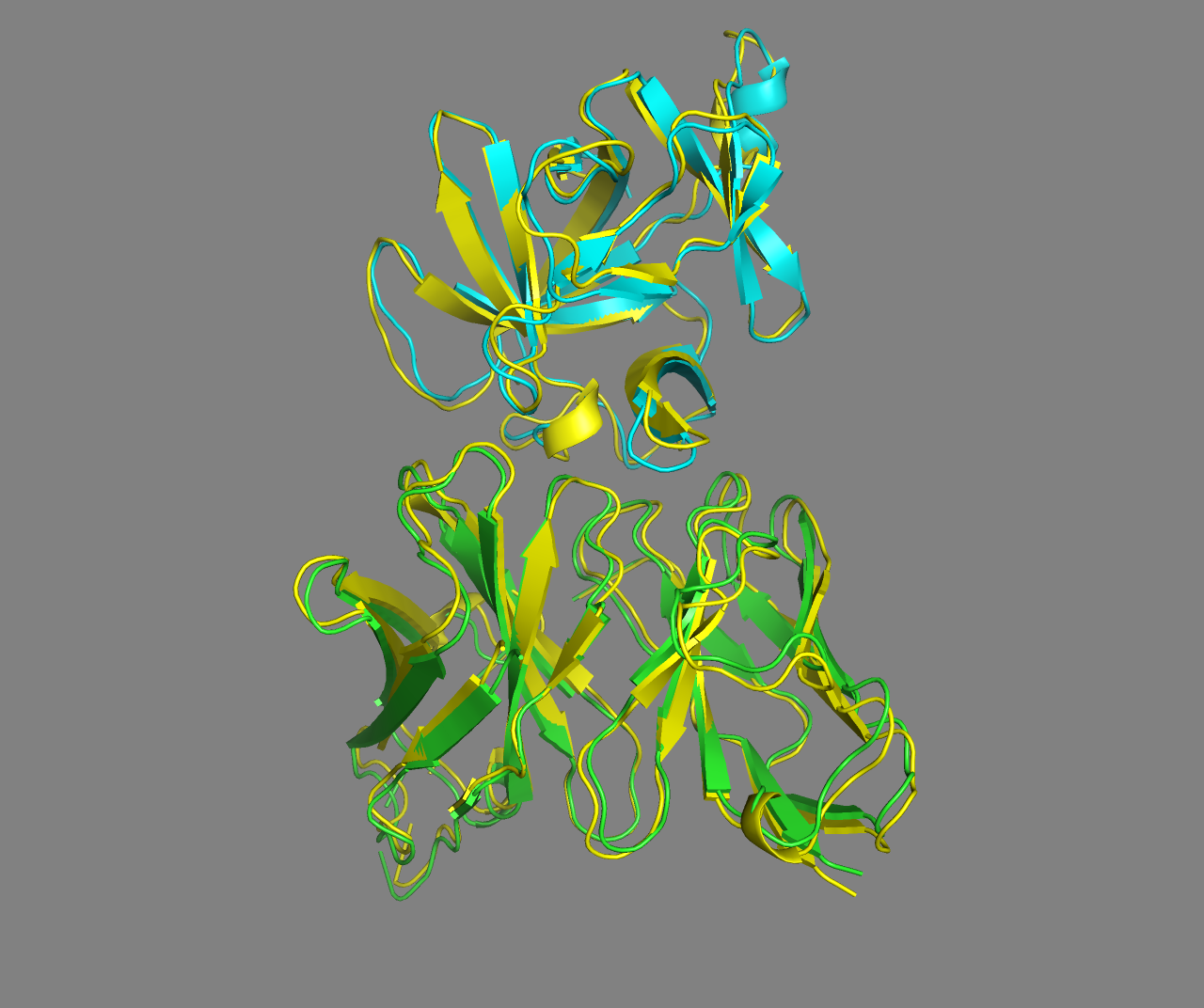
See the overlay of the best model onto the reference structure

Top4 models of the top cluster superimposed onto the reference crystal structure (in yellow)

BONUS: Does the antibody bind to a known interface of interleukin? ARCTIC-3D analysis

Gevokizumab is a highly specific antibody that targets an allosteric site of Interleukin-1β (IL-1β) in PDB file 4G6M, thus reducing its binding affinity for its substrate, interleukin-1 receptor type I (IL-1RI). Canakinumab, another antibody binding to IL-1β, has a different mode of action, as it competes directly with IL-1RI’s binding site (in PDB file 4G6J). For more details please check this article.

We will now use our new software, ARCTIC-3D, to visualize the binding interfaces formed by IL-1β. First, the program retrieves all the existing binding surfaces formed by IL-1β from the PDBe website. Then, these binding surfaces are compared and clustered together if they span a similar region of the selected protein (IL-1β in our case).

We can now open the ARCTIC-3D web-server page here. We will run an ARCTIC-3D job targeting the uniprot ID proper to human Interleukin-1 beta, namely P01584.

Insert the selected uniprot ID in the UniprotID field.

Leave the other parameters as they are and click on Submit.

Wait a few seconds for the job to complete or access a precalculated run here.

How many interface clusters were found for this protein?

Once you download the output archive, you can find the clustering information presented in the dendrogram:

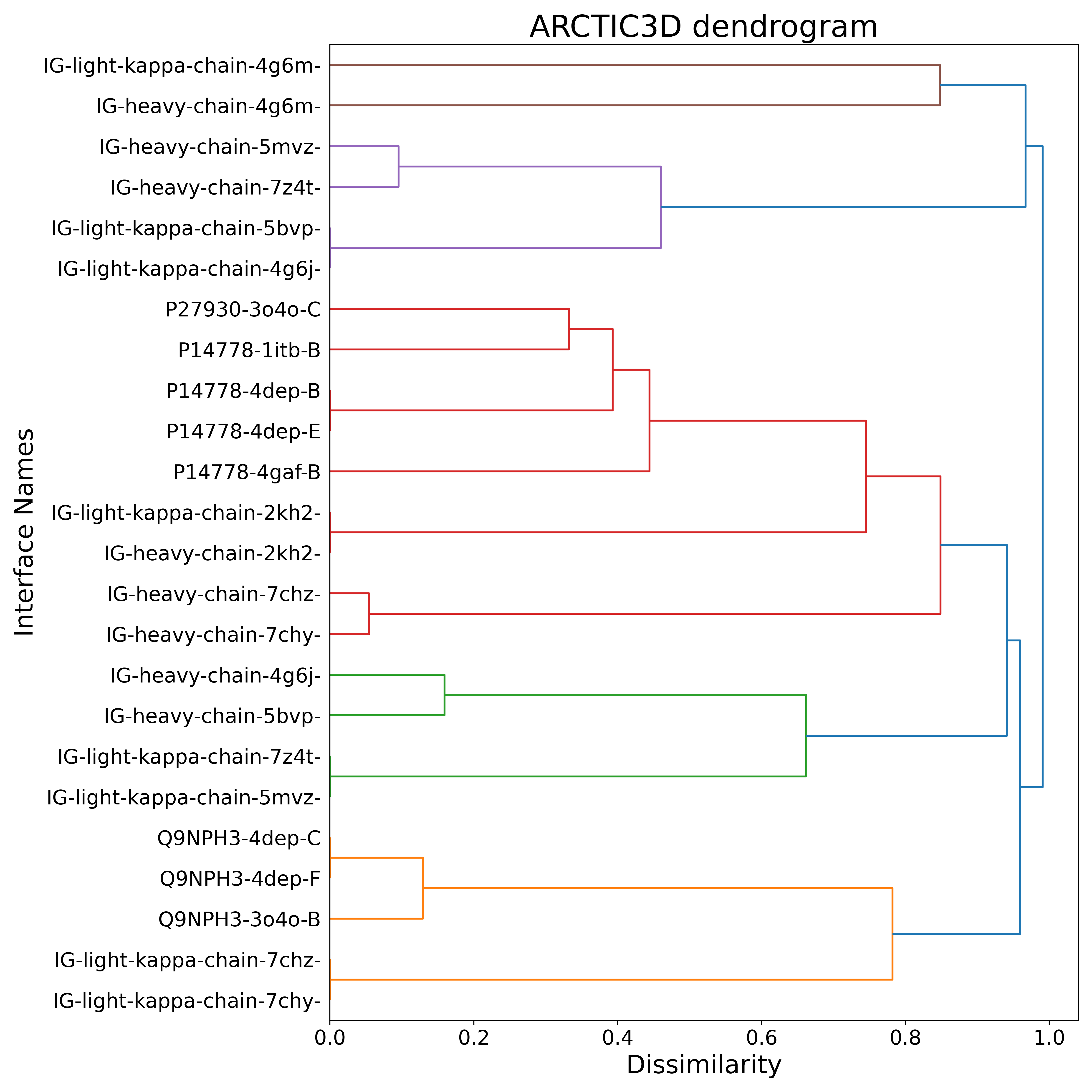
We can see how the two 4G6M antibody chains are recognized as a unique cluster, clearly separated from the other binding surfaces and, in particular, from those proper to IL-1RI (uniprot ID P14778).

Rerun ARCTIC-3D with a clustering threshold equal to 0.95

This means that the clustering will be looser, therefore lumping more dissimilar surfaces into the same object.

You can inspect a precalculated run here.

How do the results change? Are gevokizumab or canakinumab PDB files being clustered with any IL-1RI-related interface?

BONUS: Alphafold2 for antibody-antigen complex structure prediction

With the advent of Artificial Intelligence (AI) and AlphaFold we can also try to predict with AlphaFold this antibody-antigen complex.

To predict our complex, we are going to use the AlphaFold2_mmseq2 Jupyter notebook which can be found with other interesting notebooks in Sergey Ovchinnikov’s ColabFold GitHub repository, making use of the Google Colab CLOUD resources.

Start the AlphaFold2 notebook on Colab by clicking here.

Note: The bottom part of the notebook contains instructions on how to use it.

Setting up the antibody-antigen complex prediction with AlphaFold2

To setup the prediction we need to provide the sequence of the heavy and light chains of the antibody and the sequence of the antigen. These are respectively

Antibody heavy chain:

QVQLQESGPGLVKPSQTLSLTCSFSGFSLSTSGMGVGWIRQPSGKGLEWLAHIWWDGDES
YNPSLKSRLTISKDTSKNQVSLKITSVTAADTAVYFCARNRYDPPWFVDWGQGTLVTVSS

Antibody light chain:

DIQMTQSTSSLSASVGDRVTITCRASQDISNYLSWYQQKPGKAVKLLIYYTSKLHSGVPS
RFSGSGSGTDYTLTISSLQQEDFATYFCLQGKMLPWTFGQGTKLEIK

Antigen:

VRSLNCTLRDSQQKSLVMSGPYELKALHLQGQDMEQQVVFSMSFVQGEESNDKIPVALGL
KEKNLYLSCVLKDDKPTLQLESVDPKNYPKKKMEKRFVFNKIEINNKLEFESAQFPNWYI
STSQAENMPVFLGGTKGGQDITDFTMQFVSS

To use AlphaFold2 to predict e.g. the pentamer follow the following steps:

Copy and paste each of the above sequence in the query_sequence field, adding a colon : in between the sequences.

Define the jobname, e.g. Ab_Ag

In the Advanced settings block you can check the option to save the results to your Google Drive (if you have an account)

In the top section of the Colab, click: Runtime > Run All

(It may give a warning that this is not authored by Google, because it is pulling code from GitHub). This will automatically install, configure and run AlphaFold for you - leave this window open. After the prediction complete you will be asked to download a zip-archive with the results (if you configured it to use Google Drive, a result archive will be automatically saved to your Google Drive).

Time to grap a cup of tea or a coffee! And while waiting try to answer the following questions:

How do you interpret AlphaFold’s predictions? What are the predicted LDDT (pLDDT), PAE, iptm?

Tip: Try to find information about the prediction confidence at https://alphafold.ebi.ac.uk/faq. A nice summary can also be found here.

Pre-calculated AlphFold2 predictions are provided here. This archive contains the five predicted models (the naming indicates the rank), figures (png) files (PAE, pLDDT, coverage) and json files containing the corresponding values (the last part of the json files report the ptm and iptm values).

Analysis of the generated AF2 models

While the notebook is running models will appear first under the Run Prediction section, colored both by chain and by pLDDT.

The best model will then be displayed under the Display 3D structure section. This is an interactive 3D viewer that allows you to rotate the molecule and zoom in or out.

Note that you can change the model displayed with the rank_num option. After changing it execute the cell by clicking on the run cell icon on the left of it.

Consider the pLDDT of the various models (the higher the pLDDT the more reliable the model).

What is the confidence of those predictions? (check again the FAQ page of the Alphafold database provided above for pLDDT values)

While the pLDDT score is an overall measure, you can also focus on the interface score reported in the iptm score (value between 0 and 1).

See the confidence statistics for the five generated models

    Model1: pLDDT=90.4 pTM=0.654 ipTM=0.525
    Model2: pLDDT=88.0 pTM=0.65  ipTM=0.522
    Model3: pLDDT=88.2 pTM=0.647 ipTM=0.52
    Model4: pLDDT=88.0 pTM=0.644 ipTM=0.516
    Model5: pLDDT=88.1 pTM=0.641 ipTM=0.512

Based on the iptm scores, would you qualify those models as reliable?

Note that in this case the iptm score reports on all interfaces, i.e. both the interface between the two chains of the antibody, and the antibody-antigen interface

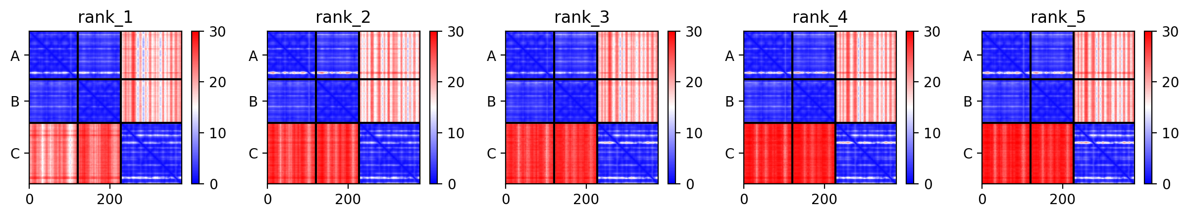
Another useful way of looking at the model accuracy is to check the Predicted Alignment Error plots (PAE) (also referred to as Domain position confidence). The PAE gives a distance error for every pair of residues: It gives AlphaFold’s estimate of position error at residue x when the predicted and true structures are aligned on residue y. Values range from 0 to 35 Angstroms. It is usually shown as a heatmap image with residue numbers running along vertical and horizontal axes and each pixel colored according to the PAE value for the corresponding pair of residues. If the relative position of two domains is confidently predicted then the PAE values will be low (less than 5A - dark blue) for pairs of residues with one residue in each domain. When analysing your complex, the diagonal block will indicate the PAE within each molecule/domain, while the off-diagonal blocks report on the accuracy of the domain-domain placement.

Our antibody-antigen complex consists of three interfaces:

The interface between the heavy and light chains of the antibody
The interface between the heavy chain of the antibody and the antigen
The interface between the light chain of the antibody and the antigen

See the PAE plots for the five generated models

Based on the PAE plots, which interfaces can be considered reliable/unreliable?

Visualization of the generated AF2 models

Let’s now visualize the models in PyMOL. For this save your predictions to disk or download the precalculated AlphaFold2 model from here.

Start PyMOL and load via the File menu all five AF2 models.

File menu -> Open -> select abagtest_2d03e_unrelaxed_rank_001_alphafold2_multimer_v3_model_3_seed_000.pdb

Repeat this for each model (abagtest_2d03e_unrelaxed_rank_X_alphafold2_multimer_v3_model_X_seed_000.pdb or whatever the naming of your model is).

Let’s superimpose all models on the antibody (the antibody in the provided AF2 models correspond to chains A and B):

util.cbc
select Ab_Ag_unrelaxed_rank_1_model_2 and chain A+B
alignto sele

This will align all clusters on the antibody, maximizing the differences in the orientation of the antigen.

Examine the various models. How does the orientation of the antigen differ between them?

Note: You can turn on and off a model by clicking on its name in the right panel of the PyMOL window.

See tips on how to visualize the prediction confidence in PyMOL

When looking at the structures generated by AlphaFold in PyMOL, the pLDDT is encoded as the B-factor.
To color the model according to the pLDDT type in PyMOL:
spectrum b **Note** that the scale in the B-factor field is the inverse of the color coding in the PAE plots: i.e. red mean reliable (high pLDDT) and blue unreliable (low pLDDT))

Since we do have NMR chemical shift perturbation data for the antigen, let’s check if the perturbed residues are at the interface in the AF2 models. Note that there is a shift in numbering of 2 residues between the AF2 and the HADDOCK models.

util.cbc
select epitope, (resi 70,71,72,73,81,82,87,88,90,92,94,95,96,113,114,115) and chain C
color orange, epitope

Does any model have the NMR-identified epitope at the interface with the antibody?

See the AlphaFold models with the NMR-mapped epitope

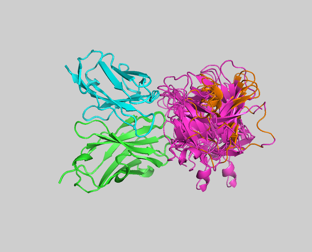
It should be clear from the visualization of the NMR-mapped epitope on the AF2 models that none does satisfy the NMR data. To further make that clear we can compare the models to the crystal structure of the complex (4G6M).

For this download and superimpose the models onto the crystal structure in PyMOL with the following commands:

fetch 4G6M
remove resn HOH
color yellow, 4G6M
select 4G6M and chain H+L
alignto sele

See the AlphaFold models superimposed onto the crystal structure of the complex (4G6M)

Conclusions

We have demonstrated the usage of HADDOCK3 in an antibody-antigen docking scenario making use of the paratope information on the antibody side (i.e. no prior experimental information) and a NMR-mapped epitope for the antigen. Compared to the static HADDOCK2.X workflow, the modularity and flexibility of HADDOCK3 allows to customise the docking protocols and to run a deeper analysis of the results. While HADDOCK3 is still very much work in progress, its intrinsic flexibility can be used to improve the performance of antibody-antigen modelling compared to the results we presented in our Structure 2020 article and in the related HADDOCK2.4 tutorial.

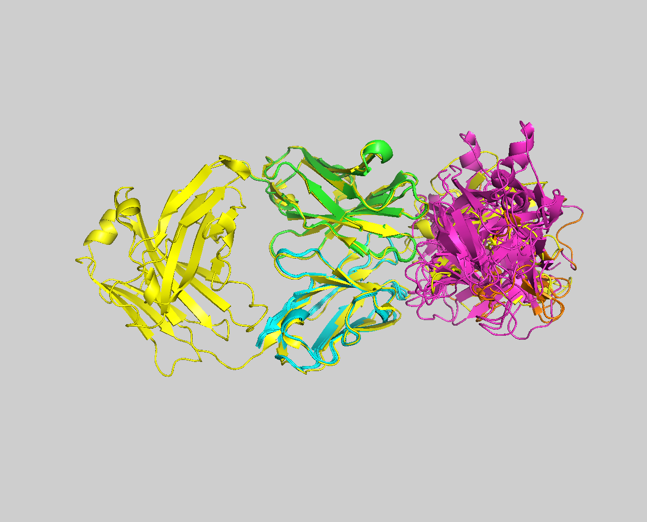
Congratulations! 🎉

You have completed this tutorial. If you have any questions or suggestions, feel free to contact us via email or asking a question through our support center.

And check also our education web page where you will find more tutorials!