

Nanobody-antigen modelling tutorial using a local version of HADDOCK3
This tutorial consists of the following sections:
- Introduction
- Setup/Requirements
- Preparing PDB files for docking
- Defining restraints for docking
- Setting up the docking with HADDOCK3
- Analysis of docking results
- Visualisation and comparison with the reference structure
- Visualising the contact map of the best clusters
- BONUS 1: design interface mutations in a nanobody-antigen complex with HADDOCK3
- Conclusions
Introduction
Nanobodies are monomeric proteins that closely resemble the variable region of the heavy chain of an antibody. They are derived from camelid heavy-chain antibodies and are composed of a single variable domain (VHH) that contains the antigen-binding site. Nanobodies are small, stable, and soluble proteins that can be easily produced in bacteria, yeast, or mammalian cells. They have a high affinity for their target antigens, typically comparable to that of monoclonal antibodies. Nanobodies are used in a wide range of applications, such as therapeutics and disease diagnosis.
As in antibodies, the small part of the nanobody region that binds the antigen is called paratope, while part of the antigen that binds to a nanobody is called epitope. Different from antibodies, nanobodies have only three complementarity-determining regions (CDRs-hypervariable loops) whose sequence and conformation are altered to bind to different antigens. Another important feature of these molecules is that the highly conserved amino acids that are not part of the CDRs, namely the framework regions (FRs), can play a role in the binding to the antigen.
Predicting the structure of a nanobody-antigen complex is very challenging, as the epitope can be located in any part of the antigen molecule. In the last years AlphaFold2-Multimer has been shown to be able to predict the correct structure of the nanobody-antigen complex for a limited number of cases. This is due to the fact that there is no co-evolution between the antibody and antigen sequences, which makes the prediction of the correct conformation extremely difficult. AlphaFold3 is expected to improve the prediction of the nanobody-antigen complex, but still fails for many cases.
This tutorial demonstrates the use of the new modular HADDOCK3 version for predicting the structure of a nanobody-antigen complex using different possible information scenarios, ranging from complete knowledge of the epitope to more limited information.
In this tutorial we will be working with the complex between a nanobody (1-2C7), and a fragment of the Severe acute respiratory syndrome coronavirus 2 (SARS-CoV-2) Spike glycoprotein (PDB ID: 7x2m).
Throughout the tutorial, colored text will be used to refer to questions or instructions, and/or PyMOL commands.
This is a question prompt: try answering it! This an instruction prompt: follow it! This is a PyMOL prompt: write this in the PyMOL command line prompt! This is a Linux prompt: insert the commands in the terminal!
Setup/Requirements
In order to follow this tutorial you will need to work on a Linux or MacOSX system. We will also make use of PyMOL (freely available for most operating systems) in order to visualize the input and output data.
We assume that you have a working installation of HADDOCK3 on your system.
In case HADDOCK3 is not pre-installed in your system you will have to install it. To obtain HADDOCK3, fill the registration form, and then follow the installation instructions.
In this tutorial we will use the PyMOL molecular visualisation system. If not already installed, download and install PyMOL from here. You can use your favourite visualisation software instead, but be aware that instructions in this tutorial are provided only for PyMOL.
Further we are providing pre-processed PDB files for docking and analysis (but the preprocessing of those files will also be explained in this tutorial). The files have been processed to facilitate their use in HADDOCK and for allowing comparison with the known reference structure of the complex. For this download and unzip the following zip archive and note the location of the extracted files in your system. In it you should find the following directories:
haddock3: Contains HADDOCK3 configuration and job files for the various scenarios in this tutorialpdbs: Contains the pre-processed PDB filesrestraints: Contains the interface information and the correspond restraint files for HADDOCKruns: Contains pre-calculated run results for the various scenarios in this tutorial
Preparing PDB files for docking
In this section we will prepare the PDB files of the nanobody and antigen for docking.
Crystal structures of both the antibody and the antigen in their free forms are available from the
PDBe database. We will use pdb-tools to perform several operations on the PDB files, such as selecting chains, renumbering residues, and creating ensembles. pdb-tools is already installed in the haddock3 environment. For more information about the requirements for pdb files in HADDOCK3, please refer to the HADDOCK3 user manual - structure requirements.
Note that pdb-tools is also available as a web service.
Note: Before starting to work on the tutorial, make sure to activate haddock3 if installed using conda
conda activate haddock3
Preparing the nanobody structural ensemble
When having to deal with a nanobody, it is quite unlikely that its structure in the “unbound” form (i.e., without the antigen attached) has already been deposited on the PDB, but it’s always good to check.
Our sequence of interest is the following:
QVQLQESGGGLVQPGGSLRLSCAASGDTLDLYAIGWFRQTPGEEREGVSCISPSGSRTNYADSVKGRFTISRDNAKNTVYLQMNGLRPEDTAVYFCAGSRPSAHYCSHYPTEYDDWGQGTQVTV
Let’s search the PDB database for similar sequences using the PDB advanced search.
Paste the nanobody sequence into the Sequence Similarity box.
Using the nanobody structure directly from the target PDB (7X2M) would not be very realistic, as the nanobody is already bound to the antigen. In a real-case scenario you would be forced to model the nanobody structure from scratch.
A possible way to do this is to use AlphaFold2. You can run your AlphaFold modelling from Colabfold.
We provide you with AlphaFold2 models coming from the nanobody run in presence (Alphafold2-multimer) and absence (AlphaFold2-monomer) of the antigen. The models are available in the pdbs directory of the archive you downloaded. Additionally, we provide you with some models coming from an antibody-specific predictor, ImmuneBuilder.
Let us have a look at them in PyMOL. If first starting PyMOL, load the PDB files as followed:
When starting PyMOL directly from the command line you can use instead:
pymol pdbs/7X2M_multimer_rank_001.pdb pdbs/7X2M_monomer_rank_001.pdb pdbs/7X2M_IB_rank_001.pdb
Remember that the ranking used by AlphaFold2 changes between the monomer and multimer version!
Are the three nanobody models different? If yes, where do you see the major differences?
The CDR3 loop is the main contributor to the binding, and it is the longest and most variable loop in the nanobody. Predicting its conformation is extremely challenging, and it is not uncommon to see different conformations in the models. Highlight CDR3 in the structure with the following PyMOL command:
select cdr3, 7X2M_monomer_rank_001.pdb and resi 99:115 color red, cdr3
It looks like the CDR3 loop is “folding back” on the nanobody framework, at least in the predicted models. This conformation, typically called “kinked”, is one of the two main observed conformations of the CDR3 loop in nanobodies. The other one is an “extended” conformation, where the loop is pointing away from the framework. Most of the nanobodies show a kinked conformation, but the extended one is not uncommon (occurs in about 30% of the cases).
Let us now visualize AlphaFold2’s confidence in the prediction and in particular the values of the predicted Local Distance Difference Test (pLDDT) score. The pLDDT score is a per-residue confidence score that ranges from 0 to 100, with higher values indicating higher confidence. In AlphaFold2 and similar predictors the confidence score is typically encoded in the B-factor column of the PDB file. To color the CDR3 loop based on the pLDDT scores type the following command in PyMOL:
See the pLDDT-coloured CDR3 loop

In this case the overall fold of the nanobody is well predicted, including the kinked region of the CDR3 loop. We cannot say much about the three/four residues at the end of the CDR3 loop (the ones in blue), as their confidence is rather low. To account for possible differences in conformations of the H3 loop, in this case we will combine the three nanobody models into a structural ensemble, with the aim of capturing a possibly correct H3 conformation in at least one of the models. This has been shown multiple times to be a good strategy to improve the docking results.
First, let’s extract the nanobody (chain A) from the multimer model using pdb-tools.
pdb_selchain -A pdbs/7X2M_multimer_rank_001.pdb > 7X2M_multimer_rank_001_A.pdb
Now we have to renumber the ImmuneBuilder model, as its numbering is not coherent with the other AlphaFold models.
pdb_reres -1 pdbs/7X2M_IB_rank_001.pdb | pdb_chain -A | pdb_tidy > 7X2M_IB_A.pdb
We can now create the ensemble.
Note that the corresponding files can be found in the pdbs directory of the archive you downloaded.
Preparing the antigen structure
Is it necessary to build the antigen structure from scratch using AlphaFold? Let us first check the PDB database. The fact that we are dealing with a fragment of an extremely well-studied protein (the Sars-CoV-2 spike protein) makes it very likely that we will find the structure of the antigen in the PDB.
The sequence of the antigen is the following:
TNLCPFGEVFNATRFASVYAWNRKRISNCVADYSVLYNSASFSTFKCYGVSPTKLNDLCFTNVYADSFVIRGDEVRQIAPGQTGNIADYNYKLPDDFTGCVIAWNSNNLDSKVGGNYNYLYRLFRKSNLKPFERDISTEIYQAGSTPCNGVKGFNCYFPLQSYGFQPTYGVGYQPYRVVVLSFELLHAPATVCGPK
We will repeat the Sequence Similarity search described above for the nanobody using the PDB advanced search:
Paste the antigen sequence into the Sequence Similarity box.
Are there any structures showing 100% sequence identity?
Using PDB-tools we will download an unbound structure of the antigen from the PDB database (the PDB ID is 7EKG).
To prepare the structure for docking, we will:
- select the chain corresponding to our antigen (
pdb_selchain), - remove any hetero atoms from the structure (e.g. crystal waters, small molecules from the crystallisation buffer and such) (
pdb_delhetatm), - remove any possible side-chain duplication (can be present in high-resolution crystal structures in case of multiple conformations of some side chains) (
pdb_selaltloc), - keep only the coordinates lines (
pdb_keepcoord), - renumber the residues starting at 1 (
pdb_reres), and - clean the PDB file (
pdb_tidy).
Note The last command pdb_tidy -strict cleans the PDB file, and adds TER statements only between different chains. Without the -strict option TER statements would be added between each chain break (e.g. missing residues), which should be avoided.
Defining restraints for docking
Before setting up the docking we need first to generate distance restraint files in a format suitable for HADDOCK. HADDOCK uses CNS as computational engine. A description of the format for the various restraint types supported by HADDOCK can be found in our Nature Protocol 2024 paper, Box 1.
Distance restraints are defined as:
assign (selection1) (selection2) distance, lower-bound correction, upper-bound correction
The lower limit for the distance is calculated as: distance minus lower-bound
correction
and the upper limit as: distance plus upper-bound correction.
The syntax for the selections can combine information about chainID - segid
keyword -, residue number - resid keyword -, atom name - name keyword.
Other keywords can be used in various combinations of OR and AND statements.
Please refer for that to the online CNS manual.
We will shortly explain in this section how to generate ambiguous interaction restraints (AIRs) in HADDOCK illustrating the following three scenarios:
- HV loops on the nanobody, epitope region on the antigen
- HV loops on the nanobody, vaguely defined epitope region on the antigen
- HV loops on the nanobody, mutagenesis-based restraints on the antigen
Information about various types of distance restraints in HADDOCK can also be found in our online manual pages.
Checking for chain breaks
When docking multi-chain proteins (treated as a single chain in HADDOCK), it is important to define unambiguous distance restraints to keep the two chains or domains together during the flexible refinement part of HADDOCK. This is done by defining a set of distance restraints between atoms of the two chains. An example of this is given by standard antibody antigen docking protocols, where the heavy and light chains are kept together by defining a few distance restraints between the C-alpha atoms of the two chains, as illustrated in the HADDOCK2.4 protein-protein tutorial and in corresponding section of the HADDOCK3 antibody-antigen tutorial.
In this tutorial, we do not need to define unambiguous restraints neither for the nanobody nor for the antigen, as they are monomeric entities.
Important, in general, it is recommended to check for the presence of chain breaks or missing segments in your protein and define unambiguous restraints to keep those together. This can be done using the haddock3-restraints restrain_bodies tool.
Identifying the paratope of the nanobody
The paratope is the region of the nanobody that binds to the antigen. In the case of nanobodies, the paratope is mainly composed of the CDR loops, but the framework regions can also play a role in the binding. The CDR3 loop is the most important one, and will for sure be part of the paratope.
Let us start by identifying all the amino acids that lie on the CDR loops and that are exposed to the surface. To do this we will use the haddock3-restraints calc_accessibility command, which calls the FreeSASA library to calculate the solvent accessible surface area of the residues.
haddock3-restraints calc_accessibility pdbs/7X2M_monomer_rank_001.pdb
This command will generate a list of residues with relative side-chain solvent accessibility larger 0.4 (default cutoff, which can be changed).
14/02/2025 16:53:53 L116 INFO - Calculate accessibility...
14/02/2025 16:53:53 L227 INFO - Chain: A - 124 residues
14/02/2025 16:53:53 L236 INFO - Applying cutoff to side_chain_rel - 0.4
14/02/2025 16:53:53 L248 INFO - Chain A - 1,3,5,7,8,10,11,13,14,15,16,17,19,23,25,26,27,28,30,31,39,41,42,43,44,46,54,56,57,59,62,63,65,66,69,71,73,75,76,77,84,85,87,88,89,100,101,102,104,105,109,111,112,114,118,121,123
Upon cross-referencing with the CDRs, we can identify the residues that are part of the paratope:
26,27,28,30,31,54,56,57,100,101,102,104,105,109,111,112,114
Let us visualize those onto the 3D structure.
For this start PyMOL and load one of the elements of the 7X2M_nb_ensemble.pdb ensemble (e.g., the monomer model).
File menu -> Open -> select 7X2M_monomer_rank_001.pdb
We will now highlight the predicted paratope. In PyMOL type the following commands:
color white, all
select paratope, (resi 26+27+28+30+31+54+56+57+100+101+102+104+105+109+111+112+114)
color red, paratope
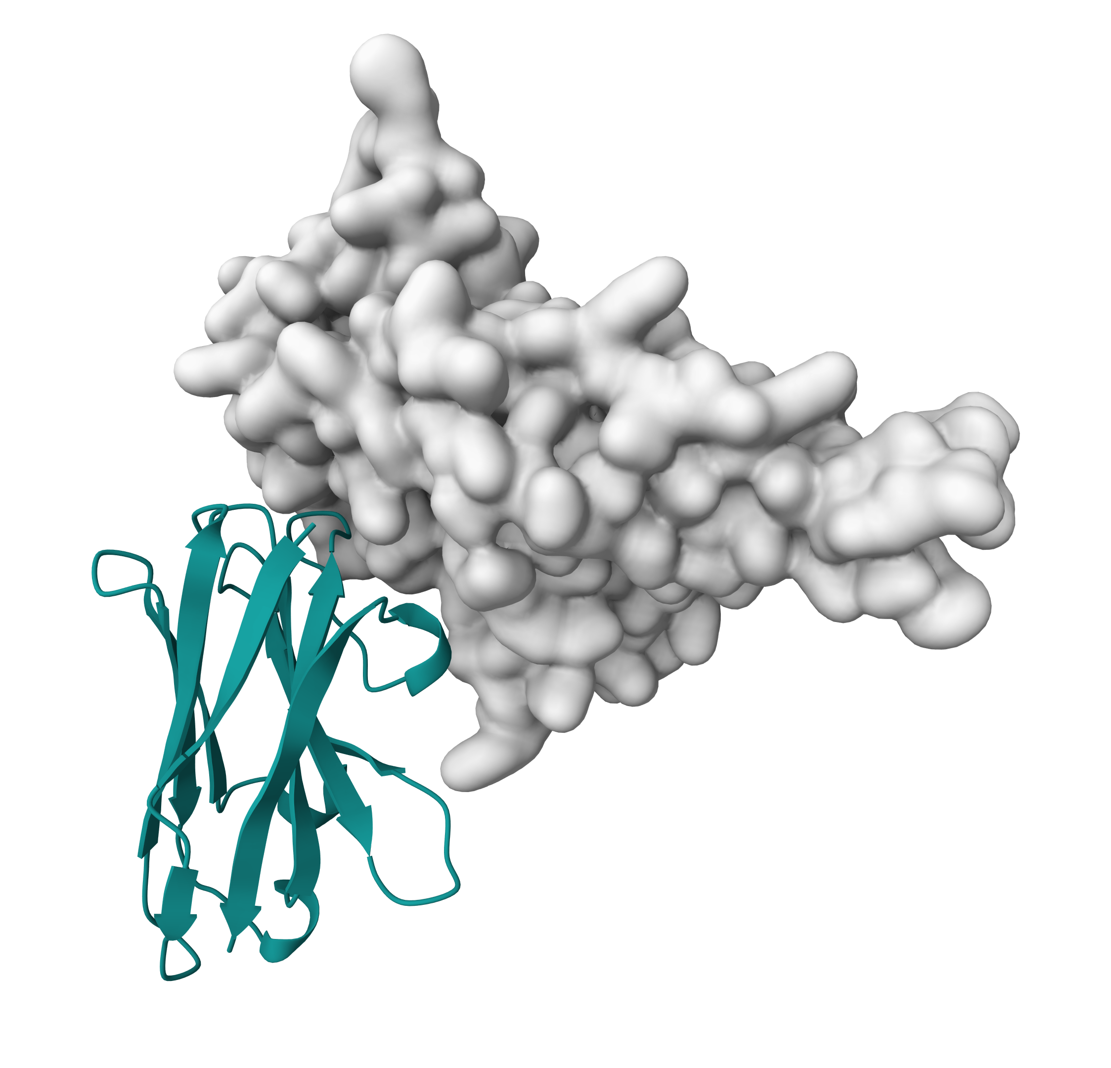
Let us now switch to a surface representation to inspect the predicted binding site.
Inspect the surface.
Do the identified residues form a well defined patch on the surface?
See surface view of the paratope expand_more
Antigen scenario 1: true epitope information
In this scenario we will assume that we have perfect knowledge of the epitope region on the antigen. This can be considered a best-case scenario, as it is quite unlikely to have such detailed information in real life. An example of this scenario is when the epitope region has been extensively mapped through NMR chemical shift titration experiments, as shown in the HADDOCK3 antibody-antigen tutorial.
The list of epitope residues is
37,38,39,40,41,42,43,44,45,46,171,172,176
Let us visualize those onto the 3D structure. For this start PyMOL and load the 7EKG_clean.pdb file.
File menu -> Open -> select 7EKG_clean.pdb
We will now highlight the epitope residues. In PyMOL type the following commands:
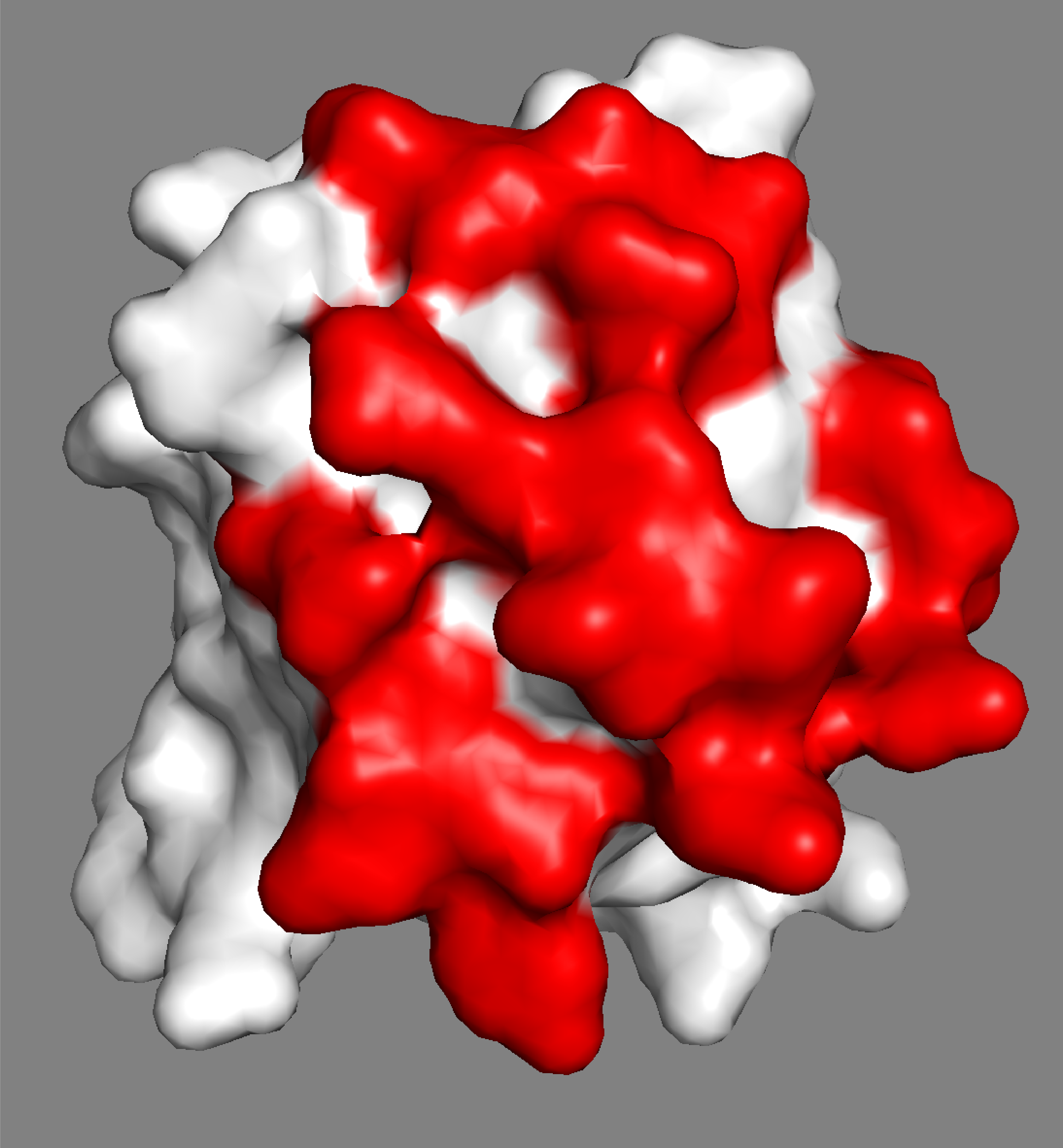
color white, all select epitope, (resi 37+38+39+40+41+42+43+44+45+46+171+172+176) color red, epitope show surface
Inspect the surface.
Do the identified residues form a well defined patch on the surface?
See surface view of the epitope expand_more

Defining ambiguous restraints for scenario 1
We will now generate the ambiguous interaction restraints (AIRs) for this scenario. The AIRs will be used to define the paratope-epitope interaction. The AIRs will be generated using the haddock3-restraints tool.
To use our haddock3-restraints active_passive_to_ambig script you need to
create for each molecule a file containing two lines:
- The first line corresponds to the list of active residues (numbers separated by spaces)
- The second line corresponds to the list of passive residues (in this scenario no passive residues are defined)
For scenario 1 this would be:
- For the antibody (the file called
antibody-cdr.actpassfrom therestraintsdirectory):
26 27 28 30 31 54 56 57 100 101 102 104 105 109 111 112 114
- For the antigen (the file called
antigen-epi.actpassfrom therestraintsdirectory):
37 38 39 40 41 42 43 44 45 46 171 172 176
We will now generate the AIR file:
This will generate the file cdr_epitope.tbl. A copy of this file is available in the restraints directory.
Antigen scenario 2: loosely-defined epitope information
In this scenario we assume that we only have a vague idea of the epitope region on the antigen, a more realistic scenario. Here the region may have been identified through competition experiments or less precise mapping techniques.
The list of epitope residues for this scenario is
32,34,35,36,37,38,39,40,41,42,43,44,45,46,47,48,50,51,52,53,54,71,72,73,104,105,169,170,171,172,173,176
We can visualize those onto the 3D structure with PyMOL as we did before:
File menu -> Open -> select 7EKG_clean.pdb
color white, all
show surface
select loose_epitope, (resi 32+34+35+36+37+38+39+40+41+42+43+44+45+46+47+48+50+51+52+53+54+71+72+73+104+105+169+170+171+172+173+176)
color red, loose_epitope
How did the epitope surface change?
For this scenario we will define this patch as passive in the docking, as we are not sure whether all the residues are part of the epitope. In fact, most of them are not part of the true epitope. Passive residues will not lead to energetic penalties when not part of the interface in the docked models.
Rule of thumb: for HADDOCK it is better to be more generous rather than too strict in the definition of the interface. The docking protocol will automatically discard 50% of the active residue restraints for every docking pose, allowing to discriminate between structurally plausible and unfavourable restraints.
Defining ambiguous restraints for scenario 2
We will now generate the AIRs for this scenario.
-
For the antibody we will keep using the same file as before (
antibody-cdr.actpassfrom therestraintsdirectory).: -
For the antigen (the file called
antigen-loose_epi.actpassfrom therestraintsdirectory):
32 34 35 36 37 38 39 40 41 42 43 44 45 46 47 48 50 51 52 53 54 71 72 73 104 105 169 170 171 172 173 176
Here the first line is empty as we are not defining any active residues for the antigen.
Generate the AIRs file with the following command:
This will generate the file cdr-loose_epi.tbl. A copy of this file is available in the restraints directory.
Antigen scenario 3: mutagenesis-based epitope information
In this scenario we assume that we have limited information about the epitope region on the antigen coming from mutagenesis experiments. This is a very common scenario in the field of structural biology, where one or two residues are known to be crucial for the binding, but the remaining of the epitope is completely unknown.
In this case our rationale is to define the two residues as active and to define the solvent-exposed residues around them as passive.
We assume that our mutagenesis-mapped residues are Tyrosine 37 and Lysine 46.
Now we will define the passive residues around those using a default relative solvent accessibility of 0.15 and an increased radius of 7.5Å (default is 6.5):
haddock3-restraints passive_from_active 7EKG_clean.pdb 37,46 -r 7.5
You should get a list of residues very similar to this one:
32 33 34 35 36 38 39 40 41 42 43 44 45 47 48 50 51 52 53 54 76 79 97
Let us visualize those onto the 3D structure using PyMOL as we did before:
File menu -> Open -> select 7EKG_clean.pdb
color white, all
select mutagenesis_active, (resi 37+46)
color red, mutagenesis_active
select mutagenesis_passive, (resi 32+33+34+35+36+38+39+40+41+42+43+44+45+47+48+50+51+52+53+54+76+79+97)
color orange, mutagenesis_passive
show sticks, mutagenesis_active
show sticks, mutagenesis_passive
See the epitope determined from mutagenesis residues expand_more

Defining ambiguous restraints for scenario 3
We will now generate the AIRs file for this scenario.
-
For the antibody we will use the same file as before (
antibody-cdr.actpassfrom therestraintsdirectory).: -
For the antigen (the file called
antigen-mut_epi.actpassfrom therestraintsdirectory):
37 46
32 33 34 35 36 38 39 40 41 42 43 44 45 47 48 50 51 52 53 54 76 79 97
Note how first line corresponds to the active residues and the second line to the passive residues.
Generate the AIRs file with the following command:
This will generate the file cdr-mut_epi.tbl. A copy of this file is available in the restraints directory.
Setting up the docking with HADDOCK3
Having now all the required restraints we can proceed with the docking setup. We will use the HADDOCK3 software to perform the docking calculations.
Defining the modelling workflow
Here we will stick to the most basic HADDOCK3 workflow, which is the literal translation of the HADDOCK2.4 workflow, but several other workflows are possible, such as adding a clustering step between the rigid-body and the semi-flexible refinement stages, as done in the HADDOCK3 antibody-antigen tutorial.
For various examples of HADDOCK3 workflows, please refer to the HADDOCK3 GitHub repository. F or nanobody-specific workflows, check out the corresponding HADDOCK3 examples.
Our workflow consists of the following steps (modules):
- topoaa: Generates the topologies for the CNS engine and builds missing atoms
- rigidbody: Performs rigid body energy minimisation (
it0in HADDOCK2.X) - caprieval: Calculates CAPRI metrics (i-RMSD, l-RMSD, Fnat, DockQ) with respect to the top scoring model or reference structure if provided
- seletop : Selects the top N models from the previous module
- flexref: Performs semi-flexible refinement of the interface (
it1in HADDOCK2.X) - caprieval
- emref: Final refinement by energy minimisation (
itwEM only in HADDOCK2.X) - caprieval
- clustfcc: Clustering of models based on the fraction of common contacts (FCC)
- seletopclusts: Selects the top models of all clusters
- caprieval
- contactmap: Contacts matrix and a chordchart of intermolecular contacts
The configuration file for the three scenarios is already provided in the haddock3 directory of the archive you downloaded.
If we consider the first scenario, the workflow is as follows (file haddock3/nanobody-antigen-real.cfg):
#================== General parameters, input files and settings ==========
# execution mode
mode = "local"
# run directory
run_dir = "./run-real-unbound-7ekg"
# number of cores to use
ncores = 24
# input molecules, AI-derived nanobody ensemble and antigen from the PDB
molecules = [
    "./pdbs/7X2M_nb_ensemble.pdb",
    "./pdbs/7EKG_clean.pdb",
]

#================== Workflow definition ===================================

[topoaa]

[rigidbody]
ambig_fname = "./restraints/cdr_epitope.tbl"

[caprieval]
reference_fname = "./pdbs/7x2mB_ref.pdb"

[seletop]
select = 200

[flexref]
tolerance = 10
ambig_fname = "./restraints/cdr_epitope.tbl"
# in the case of unambiguous restraints, uncomment this line
# and link the correct file
# unambig_fname = "./restraints/7x2mB_unambig.tbl"

[caprieval]
reference_fname = "./pdbs/7x2mB_ref.pdb"

[emref]
ambig_fname = "./restraints/cdr_epitope.tbl"

[caprieval]
reference_fname = "./pdbs/7x2mB_ref.pdb"

[clustfcc]

[seletopclusts]
top_models = 4

[caprieval]
reference_fname = "./pdbs/7x2mB_ref.pdb"

[contactmap]

#=========================================================================
Here we selected the local running mode and a quite high number of cores (ncores = 24) to speed up the calculations. For more information about HADDOCK running modes please check the documentation or the corresponding section in the antibody-antigen tutorial. If you are running the tutorial on your laptop, you will not have access to so many cores, and HADDOCK will automatically adjust the number of cores to the available ones. We recommend running this tutorial on a HPC system or on a powerful workstation.
HADDOCK3 provides an analysis module (caprieval) that allows
to compare models to either the best scoring model (if no reference is given) or to a reference structure, which in our case we have at hand (7x2mB_ref.pdb).
Decreasing sampling to limit the computing time
When running locally with limited computational resources, you can adjust a few parameters to make the execution faster. For example, you can reduce the number of models generated in the rigid-body docking stage by changing the sampling parameter in the rigidbody section of the configuration file. The default value is 1000, but you can put it to 100 or 200 to generate fewer models. At the same time you can also reduce the number of rigid-body models selected for refinement, e.g. 50, in the seletop section.
...
[topoaa]

[rigidbody]
ambig_fname = "./restraints/7x2mB_real_ambig.tbl"
sampling = 200

[caprieval]
reference_fname = "./pdbs/7x2mB_ref.pdb"

[seletop]
select = 50

[flexref]
...
These modifications will speed up the calculations substantially, but keep in mind that the quality of the results will be affected as the sampling is more limited.
Running HADDOCK
To run the docking (in local mode), simply execute the following command:
haddock3 ./haddock3/nanobody-antigen-real.cfg
This will start the docking calculations. The output will be stored in the run-real-unbound-7ekg directory.
The same procedure can be followed for the other two scenarios, by changing the configuration file accordingly.
haddock3 ./haddock3/nanobody-antigen-loose.cfg
haddock3 ./haddock3/nanobody-antigen-mut.cfg
Note that reduced sampling version of these workflows are available in the haddock3 directory, with an additional -reduced in their filename.
If you do not wish to wait for the run to finish, you can find the results of the runs in the runs/ directory of the archive you downloaded.
Analysis of docking results
Inspecting the results of the docking run
Once your run has completed inspect the content of the resulting directory. You will find the various steps (modules) of the defined workflow numbered sequentially, e.g.:
> ls run-real-unbound-7ekg/
  00_topoaa
  01_rigidbody
  02_caprieval
  03_seletop
  04_flexref
  05_caprieval
  06_emref
  07_caprieval
  08_clustfcc
  09_seletopclusts
  10_caprieval
  11_contactmap
  analysis
  data
  log
  traceback
There is in addition to the various modules defined in the config workflow a log file (text file) and three additional directories:
- the
datadirectory containing the input data (PDB and restraint files) for the various modules - the
analysisdirectory containing various plots to visualise the results for eachcaprievalstep - the
tracebackdirectory containing the names of the generated models for each step, allowing to trace back a model throughout the various stages.
You can find information about the duration of the run at the bottom of the log file. Each sampling/refinement/selection module will contain PDB files.
For example, the 09_seletopclusts directory contains the selected models from each cluster. The clusters in that directory are numbered based
on their rank, i.e. cluster_1 refers to the top-ranked cluster. Information about the origin of these files can be found in that directory in the seletopclusts.txt file.
Finding ranking, scores and model quality information
The simplest way to extract ranking information and the corresponding HADDOCK scores is to look at the X_caprieval directories
(which is why it is a good idea to have it as the final module, and possibly as intermediate steps, even when no reference structures are known).
This directory will always contain a capri_ss.tsv file, which contains the model names, rankings and statistics (score, iRMSD, Fnat, lRMSD, ilRMSD and dockq score).
The ranking in this file is based on the HADDOCK score (column 4).
E.g.:
model                         md5 caprieval_rank  score         irmsd    fnat   lrmsd   ilrmsd  dockq      cluster_id      cluster_ranking model-cluster_ranking   air     angles     bonds   bsa     cdih    coup    dani    desolv  dihe    elec    improper   rdcs    rg      sym     total   vdw     vean    xpcs
cluster_1_model_1.pdb       -       1       -88.419 2.688   0.479   9.389   5.908   0.389   3.206   3       1       1       127.812 0.000   0.000   1588.840        0.000   0.000      0.000   -4.268  0.000   -243.259        0.000   0.000   0.000   0.000   -163.728        -48.280 0.000   0.000
cluster_6_model_1.pdb       -       2       -84.588 3.545   0.417   13.407  8.407   0.285   4.228   10      6       1       91.272  0.000   0.000   1350.300        0.000   0.000      0.000   -2.488  0.000   -191.631        0.000   0.000   0.000   0.000   -153.260        -52.901 0.000   0.000
cluster_2_model_1.pdb       -       3       -83.383 9.311   0.167   29.532  20.445  0.089   9.131   4       2       1       79.337  0.000   0.000   1523.910        0.000   0.000      0.000   2.255   0.000   -209.896        0.000   0.000   0.000   0.000   -182.151        -51.592 0.000   0.000
cluster_5_model_1.pdb       -       4       -82.609 8.992   0.146   41.070  24.802  0.071   9.715   11      5       1       38.601  0.000   0.000   1474.010        0.000   0.000      0.000   -0.927  0.000   -172.699        0.000   0.000   0.000   0.000   -185.100        -51.002 0.000   0.000
cluster_1_model_2.pdb       -       5       -81.766 1.303   0.667   2.630   2.068   0.716   1.097   3       1       2       106.269 0.000   0.000   1292.000        0.000   0.000      0.000   -9.242  0.000   -222.905        0.000   0.000   0.000   0.000   -155.205        -38.570 0.000   0.000
....
The iRMSD, lRMSD and Fnat metrics are the ones used in the blind protein-protein prediction experiment CAPRI (Critical PRediction of Interactions).
In CAPRI the quality of a model is defined as (for protein-protein complexes):
- acceptable model: i-RMSD < 4Å or l-RMSD<10Å and Fnat > 0.1 (or DockQ > 0.23)
- medium quality model: i-RMSD < 2Å or l-RMSD<5Å and Fnat > 0.3 (or DockQ > 0.49)
- high quality model: i-RMSD < 1Å or l-RMSD<1Å and Fnat > 0.5 (or DockQ > 0.8)
You can use DockQ, a combination of i-RMSD, l-RMSD, and Fnat to assess the quality of the models.
It corresponds to column 9 in the capri_ss.tsv file. Since DockQ is the column number nine in the caprieval files…
What is based on this criterion the quality of the top ranked model listed above (cluster_1_model_1.pdb)? What is based on this criterion the quality of the fifth ranked model listed above (cluster_1_model_2.pdb)?
From the name of those two file we can see they belomg to the same cluster, showing that within one cluster models can show quite some variation. An analysis per cluster is discussed further down in the tutorial.
We can also find out what is the best model generated in terms of DockQ score by sorting the file based on column 9 (DockQ):
sort -r -k9 run-real-unbound-7ekg/10_caprieval/capri_ss.tsv | head -4
What is the quality of the best generated model? What is its rank?
Impact of the refinement
Since in this tutorial we do have the reference structure of the complex, we can assess and compare the quality of the models before (rigidbody) and after flexible refinement.
For this we find the best quality models by sorting the capri_ss.tsv files based on the DockQ score (column 9).
The following commands will extract the best 3 models based on the DockQ score.
After rigidbody docking:
sort -r -k9 run-real-unbound-7ekg/02_caprieval/capri_ss.tsv | head -4
After semi-flexible refinement (flexref):
sort -r -k9 run-real-unbound-7ekg/05_caprieval/capri_ss.tsv | head -4
After the final energy minimization (emef):
sort -r -k9 run-real-unbound-7ekg/07_caprieval/capri_ss.tsv | head -4
Visualising the scores and their components
The HADDOCK3 analysis precalculated a lot of plots and tables for you to inspect the results.
You can find them in the analysis directory of each run, with one folder available for each caprieval step.
The plots are in html format and can be opened in your browser. You can also open the full report in your browser:
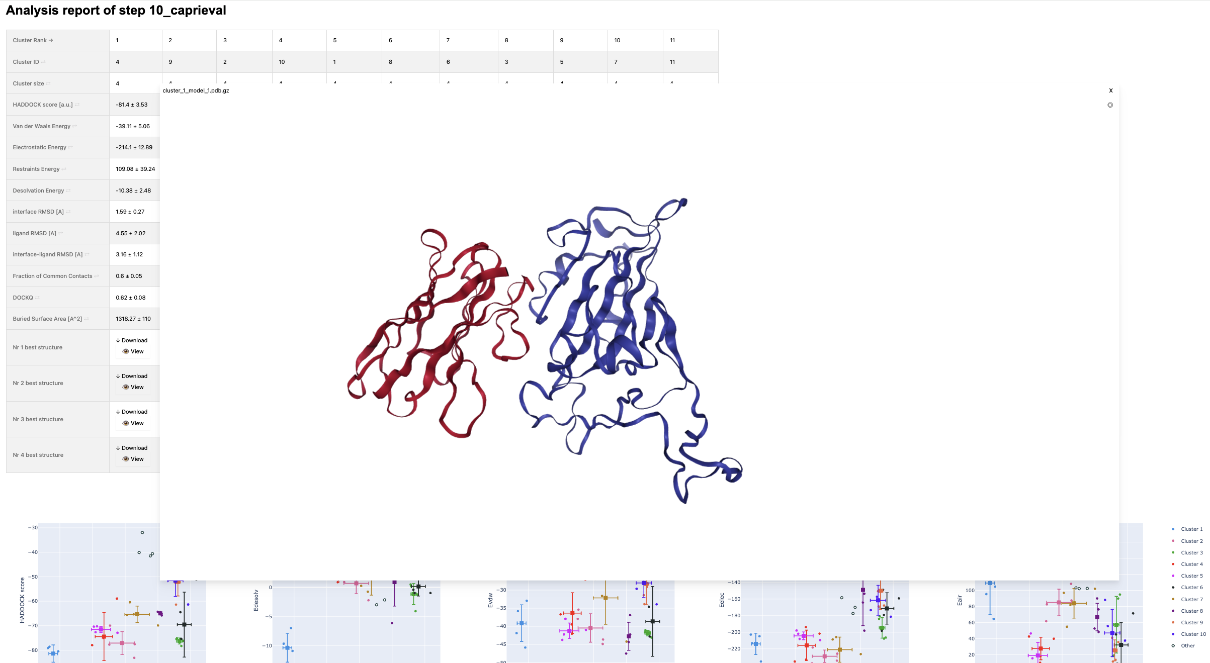
For example, to inspect the final results (after refinement):
open run-real-unbound-7ekg/analysis/10_caprieval_analysis/report.html
Cluster statistics
The clustfcc module performs the fraction of common contacts (FCC)-based clustering of the models.
Models inside a cluster are supposed to share a high number of similar contacts with the antigen, meaning that they will also be highly structurally similar.
The seletopclusts module then selects the top models from each cluster.
Let’s first see how statistically significant are the difference in scores between the different clusters.
The 10_caprieval folder contains a file named capri_clt.tsv, which contains the average and standard deviation of the scores for each cluster. Let’s inspect the file for the real interface scenario:
head -15 run-real-unbound-7ekg/10_caprieval/capri_clt.tsv
cluster_rank cluster_id n     score   score_std   irmsd   irmsd_std fnat    fnat_std lrmsd   lrmsd_std dockq   dockq_std
1            3          4     -81.125 4.668       1.726   0.580     0.557   0.081    4.868   2.893     0.592   0.136
2            4          4     -75.467 4.585       9.552   0.435     0.161   0.009    30.395  1.005     0.086   0.003
3            1          4     -74.485 5.777       4.551   0.524     0.193   0.047    19.325  3.497     0.156   0.039
4            5          4     -72.457 4.393       4.334   0.204     0.214   0.034    14.976  0.659     0.188   0.016
....
This can also be done directly from the report file.
Visualisation and comparison with the reference structure
To visualize the models from top cluster of your favorite run, start PyMOL and load the cluster representatives you want to view,
e.g. this could be the top model from cluster1. These can be found in the runs/run-real-unbound-7ekg/09_seletopclusts/ directory. Each run has a similar directory.
Let us unzip the files:
gunzip -d run-real-unbound-7ekg/09_seletopclusts/cluster_*.pdb.gz
You can load the models from the run-real-unbound-7ekg/09_seletopclusts/ directory in PyMOL.
Will first check the top ranked cluster to see if this is good solution.
File menu -> Open -> cluster_1_model_1.pdb
If you want to get an impression of how well defined a cluster is, repeat this for the best N models you want to view (cluster_1_model_X.pdb).
From the pdbs directory we can load the reference structure:
File menu -> Open -> 7x2mB_ref.pdb
Once all files have been loaded, type in the PyMOL command window:
util.cbc
color yellow, 7x2mB_ref
Let us then superimpose all models on the antigen of the reference structure:
This will use both chains to align the models, thus giving you the the full-structure RMSD with respect to the reference. Please refer to the capri files for the individual i-RMSD and l-RMSD values or try to use the rms_cur command.
To maximize the differences you can superimpose all models using a single chain. For example to fit all models on the antigen of the reference structure use:
Visualising the contact map of the best clusters
The contactmap module performs a contact analysis of the interface between the two partners. For each cluster, HADDOCK3 will analyse the existing interface contacts, providing two interactive visualizations of the contact map. In the heatmap, you can see the classical contact map, where the probability of contacts (<5A) between two residues (both intramolecular and intermolecular) are shown. The chordchart instead shows only the intermolecular contacts between the two partners, provinging type and features of the contacts.
Let’s visualize an example chordchart for the best cluster:

Check out the interactive version of the chordchart.
You can find all the contact maps in the 11_contactmap directory of the run.
BONUS 1: design interface mutations in a nanobody-antigen complex with HADDOCK3
HADDOCK3 can also be used to analyse and extract information from a nanobody-antigen complex.
We’ve already seen how to analyse the nature and type of interface contacts using the contactmap module. Now we will use HADDOCK3 to estimate the impact of mutations at the interface of a nanobody-antigen complex using the alascan module, for example to design a mutation that slightly destabilizes the complex.
The alascan module will mutate every residue at the interface into the desired amino acid (alanine by default). Although the HADDOCK score is not a predictor of binding affinity, it can be used to estimate the impact of mutations on the local environment from an energetical perspective.
Take this example HADDOCK3 workflow:
#================== General parameters, input files and settings ==========
# execution mode
mode = "local"
# run directory
run_dir = "./run-7x2m-analysis"
# number of cores to use
ncores = 1
# input molecule: here we use the reference structure, but one can use any
# other structure (or ensemble) as long as it contains the same residues
molecules = "../pdbs/7x2mB_ref.pdb"

#================== Workflow definition ===================================

[topoaa]

[emscoring]

[alascan]
plot = true

[alascan]
scan_residue = "GLY"
plot = true
#=========================================================================
With this workflow we will mutate all the interface residues to alanine and then to glycine (in the second alascan step). The alascan module will generate a plot with the difference between the scores of the wild-type and mutant structures. The scan_residue parameter allows to specify the scanning residue with a three-letter code. The default is alanine.
To run the analysis, execute the following command:
haddock3 ./haddock3/nanobody-antigen-analysis.cfg
Let’s inspect the alanine-scanning plot and the glycine-scanning plot.
Which amino acid shows the most significant impact on the antigen (chain B)?
Let’s visualize the residue ASP114 on the nanobody with pyMOL:
File menu -> Open -> 7x2mB_ref.pdb
util.cbc
select asp114, (resi 114 and chain A)
show sticks, asp114
util.cbao asp114
Now we want to visualize the interaction of this residue with the antigen.
select asp114_neighbors, (resi 114 and chain A) around 6 and chain B
show sticks, asp114_neighbors
util.cbao asp114_neighbors
if we zoom into the interaction…
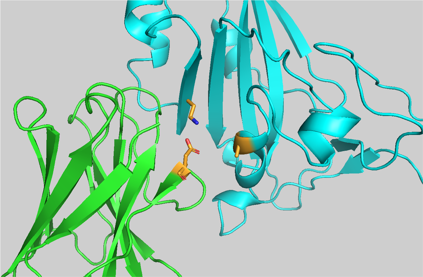
we can see a strong electrostatic interaction between ASP114 and LYS46 of the antigen. It is reasonable to expect that subsitituting ASP114 with an alanine would have a significant impact on the binding affinity of the nanobody to the antigen, thus destabilizing the complex.
Now that we idenfitied a possible key residue, we could test all the possible mutations:
mode = "local"
run_dir = "./run-7x2m-analysis-asp114"
ncores = 1
molecules = "../pdbs/7x2mB_ref.pdb"

[topoaa]

[emscoring]

[alascan]
resdic_A = [114]

[alascan]
scan_residue = "GLY"
resdic_A = [114]

[alascan]
scan_residue = "ARG"
resdic_A = [114]

[alascan]
scan_residue = "LYS"
resdic_A = [114]

...
Conclusions
We have demonstrated the usage of HADDOCK3 in a nanobody-antigen modelling and docking scenario, showing how to incorporate different levels of information on the antigen side. The use of AI-derived nanobody models allows to model the system from sequence, thus eliminating the need of an unbound nanobody structure (rarely available).
We have shown how to define ambiguous restraints for the docking, and how to set up the docking run using the HADDOCK3 software. We have also shown how to analyze the results of the docking run.
A benchmarking study of HADDOCK3 on a nanobody-antigen system has been published in biorxiv. Please refer to this publication for more information on the performance of HADDOCK3 on nanobody-antigen systems. If you use HADDOCK in your nanobody-focused research, please cite this publication.
If you want to ask questions and receive feedback don’t hesitate to contact us at the Bioexcel HADDOCK forum.
Another use case for nanobody antigen docking is the HADDOCK nanobody-antigen example in the HADDOCK3 GitHub repository, which contains similar workflows applied to a different system.