NMR and Molecular Modelling practical - HADDOCK2.4 protein-protein docking

This computer practical consists of the following sections:

Introduction
Setup
HADDOCK general concepts
Inspecting and preparing E2A for docking
Inspecting and preparing HPR for docking
Adding a phosphate group
Setting up the docking run
Analysing the results
Visualisation
Biological insights
Comparison with the reference structure
Congratulations!
Your report
Submitting your report

Introduction

This practical will demonstrate the use of HADDOCK for predicting the structure of a protein-protein complex from NMR chemical shift perturbation (CSP) data. Namely, you will dock two E. coli proteins involved in glucose transport: the glucose-specific enzyme IIA (E2A) and the histidine-containing phosphocarrier protein (HPr). The structures in the free form have been determined using X-ray crystallography (E2A) (PDB ID 1F3G) and NMR spectroscopy (HPr) (PDB ID 1HDN). The structure of the native complex has also been determined with NMR (PDB ID 1GGR). These NMR experiments have also provided us with an array of data on the interaction itself. For this tutorial, you will only make use of interface residues identified from NMR chemical shift perturbation data as described in Wang et al, EMBO J (2000).

For this tutorial you will make use of the HADDOCK2.4 webserver.

A description of the previous major version of our web server HADDOCK2.2 can be found in the following publications:

G.C.P van Zundert, J.P.G.L.M. Rodrigues, M. Trellet, C. Schmitz, P.L. Kastritis, E. Karaca, A.S.J. Melquiond, M. van Dijk, S.J. de Vries and A.M.J.J. Bonvin. The HADDOCK2.2 webserver: User-friendly integrative modeling of biomolecular complexes. J. Mol. Biol., 428, 720-725 (2015).
S.J. de Vries, M. van Dijk and A.M.J.J. Bonvin. The HADDOCK web server for data-driven biomolecular docking. Nature Protocols, 5, 883-897 (2010). Download the final author version here.

Throughout the practical, coloured text will be used to refer to questions or instructions, and/or PyMOL commands.

This is a question prompt: try answering it! This an instruction prompt: follow it! This is a PyMOL prompt: write this in the PyMOL command line prompt!

You are expected to submit a report providing answers to all questions throughout this tutorial.

Setup

In order to run this practical you will need to have the following software installed: PyMOL.

Also, if not provided with special workshop credentials to use the HADDOCK portal, make sure to register in order to be able to submit jobs. Use for this the following registration page: https://bianca.science.uu.nl/auth/register/haddock.

HADDOCK general concepts

HADDOCK (see http://www.bonvinlab.org/software/haddock2.2/) is a collection of python scripts derived from ARIA (http://aria.pasteur.fr) that harness the power of CNS (Crystallography and NMR System – http://cns-online.org) for structure calculation of molecular complexes. What distinguishes HADDOCK from other docking software is its ability, inherited from CNS, to incorporate experimental data as restraints and use these to guide the docking process alongside traditional energetics and shape complementarity. Moreover, the intimate coupling with CNS endows HADDOCK with the ability to actually produce models of sufficient quality to be archived in the Protein Data Bank.

A central aspect to HADDOCK is the definition of Ambiguous Interaction Restraints or AIRs. These allow the translation of raw data such as NMR chemical shift perturbation or mutagenesis experiments into distance restraints that are incorporated in the energy function used in the calculations. AIRs are defined through a list of residues that fall under two categories: active and passive. Generally, active residues are those of central importance for the interaction, such as residues whose knockouts abolish the interaction or those where the chemical shift perturbation is higher. Throughout the simulation, these active residues are restrained to be part of the interface, if possible, otherwise incurring in a scoring penalty. Passive residues are those that contribute for the interaction, but are deemed of less importance. If such a residue does not belong in the interface there is no scoring penalty. Hence, a careful selection of which residues are active and which are passive is critical for the success of the docking. The docking protocol of HADDOCK was designed so that the molecules experience varying degrees of flexibility and different chemical environments, and it can be divided in three different stages, each with a defined goal and characteristics:

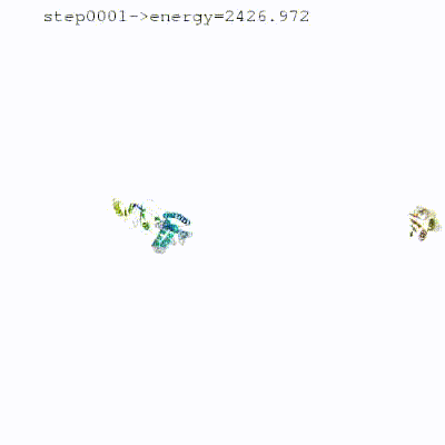
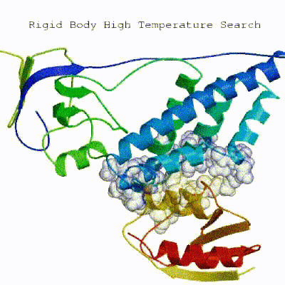
1. Randomization of orientations and rigid-body minimization (it0)
In this initial stage, the interacting partners are treated as rigid bodies, meaning that all geometrical parameters such as bonds lengths, bond angles, and dihedral angles are frozen. The partners are separated in space and rotated randomly about their centres of mass. This is followed by a rigid body energy minimization step, where the partners are allowed to rotate and translate to optimize the interaction. The role of AIRs in this stage is of particular importance. Since they are included in the energy function being minimized, the resulting complexes will be biased towards them. For example, defining a very strict set of AIRs leads to a very narrow sampling of the conformational space, meaning that the generated poses will be very similar. Conversely, very sparse restraints (e.g. the entire surface of a partner) will result in very different solutions, displaying greater variability in the region of binding.

See animation of rigid-body minimization (it0):

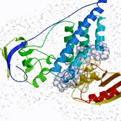
2. Semi-flexible simulated annealing in torsion angle space (it1)
The second stage of the docking protocol introduces flexibility to the interacting partners through a three-step molecular dynamics-based refinement in order to optimize interface packing. It is worth noting that flexibility in torsion angle space means that bond lengths and angles are still frozen. The interacting partners are first kept rigid and only their orientations are optimized. Flexibility is then introduced in the interface, which is automatically defined based on an analysis of intermolecular contacts within a 5Å cut-off. This allows different binding poses coming from it0 to have different flexible regions defined. Residues belonging to this interface region are then allowed to move their side-chains in a second refinement step. Finally, both backbone and side-chains of the flexible interface are granted freedom. The AIRs again play an important role at this stage since they might drive conformational changes.

See animation of semi-flexible simulated annealing (it1):

3. Refinement in Cartesian space with explicit solvent (water)
Note: This stage was part of the standard HADDOCK protocol up to (and including) v2.2. As of v2.4 it is no longer performed by default but the user still has the option of enabling it. In its place, a short energy minimisation is performed instead. The final stage of the docking protocol immerses the complex in a solvent shell so as to improve the energetics of the interaction. HADDOCK currently supports water (TIP3P model) and DMSO environments. The latter can be used as a membrane mimic. In this short explicit solvent refinement the models are subjected to a short molecular dynamics simulation at 300K, with position restraints on the non-interface heavy atoms. These restraints are later relaxed to allow all side chains to be optimized.

See animation of refinement in explicit solvent (water):

The performance of this protocol of course depends on the number of models generated at each step. Few models are less probable to capture the correct binding pose, while an exaggerated number will become computationally unreasonable. The standard HADDOCK protocol generates 1000 models in the rigid body minimization stage, and then refines the best 200 – regarding the energy function - in both it1 and water. Note, however, that while 1000 models are generated by default in it0, they are the result of five minimization trials and for each of these the 180º symmetrical solution is also sampled. Effectively, the 1000 models written to disk are thus the results of the sampling of 10.000 docking solutions. The final models are automatically clustered based on a specific similarity measure - either the positional interface ligand RMSD (iL-RMSD) that captures conformational changes about the interface by fitting on the interface of the receptor (the first molecule) and calculating the RMSDs on the interface of the smaller partner, or the fraction of common contacts (current default) that measures the similarity of the intermolecular contacts. For RMSD clustering, the interface used in the calculation is automatically defined based on an analysis of all contacts made in all models.

Inspecting and preparing E2A for docking

We will now inspect the E2A structure. For this start PyMOL and in the command line window of PyMOL (indicated by PyMOL>) type:

fetch 1F3G
show cartoon
hide lines
show sticks, resn HIS

You should see a backbone representation of the protein with only the histidine side-chains visible. Try to locate the histidines in this structure.

Q1: Is there any phosphate group present in the E2A structure? (PDB code: 1F3G). If so, state the residue name and the residue number.

Hint : you can select phosphate atoms with the following PyMOL command: select elem P

Note that you can zoom on the histidines by typing in PyMOL:

zoom resn HIS

Revert to a full view with:

zoom vis

As a preparation step before docking, it is advised to remove any irrelevant water and other small molecules (e.g. small molecules from the crystallisation buffer), however do leave relevant co-factors if present. For E2A, the PDB file only contains water molecules. You can remove those in PyMOL by typing:

remove resn HOH

Now let’s vizualize the residues affected by binding as identified by NMR. From Wang et al, EMBO J (2000) the following residues of E2A were identified has having significant chemical shift perturbations:

38,40,45,46,69,71,78,80,94,96,141

We will now switch to a surface representation of the molecule and highlight the NMR-defined interface. In PyMOL type the following commands:

color white, all
show surface
select e2a_active, (1F3G and resi 38,40,45,46,69,71,78,80,94,96,141)
color red, e2a_active

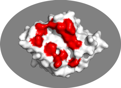
Inspect the surface.

Q2: Do the E2A residues identified by NMR as putative binding form a well-defined patch on the surface? Do they form a contiguous patch? Motivate your answers.

As final step save the molecule as a new PDB file which we will call: e2a_1F3G.pdb
For this in the PyMOL menu on top select:

File -> Save molecule… Select 1F3G and click on the save button Name your file e2a_1F3G.pdb, make sure to select PDB as format and note the location of the saved file

After saving the molecule delete it from the Pymol window or close Pymol. You can remove the molecule by typing this into the command line window of PyMOL:

delete 1F3G

Inspecting and preparing HPR for docking

We will now inspect the HPR structure. For this start PyMOL and in the command line window of PyMOL type:

fetch 1HDN
show cartoon
hide lines

Since this is an NMR structure it does not contain any water molecules and we don’t need to remove them.

Let’s vizualize the residues affected by binding as identified by NMR. From Wang et al, EMBO J (2000) the following residues were identified has having significant chemical shift perturbations:

15,16,17,20,48,49,51,52,54,56

We will now switch to a surface representation of the molecule and highlight the NMR-defined interface. In PyMOL type the following commands:

color white, all
show surface
select hpr_active, (1HDN and resi 15,16,17,20,48,49,51,52,54,56)
color red, hpr_active

Again, inspect the surface.

Q3: Do the HpR residues identified by NMR as putative binding form a well-defined patch on the surface? Do they form a contiguous patch? Motivate your answers?

Now since this is an NMR structure, it actually consists of an ensemble of models. HADDOCK can handle such ensemble, using each conformer in turn as starting point for the docking. We however recommend to limit the number of conformers used for docking, since the number of conformer combinations of the input molecules might explode (e.g. 10 conformers each will give 100 starting combinations and if we generate 1000 ridig body models (see HADDOCK general concepts above) each combination will only be sampled 10 times).

Now let’s vizualise this NMR ensemble. In PyMOL type:

hide all
show ribbon
set all_states, on

You should now be seing the 30 conformers present in this NMR structure. Let’s look at the side-chains of the active residues:

show lines, hpr_active

Q4: In contrast to E2A, HPR consists of an ensemble of models. Does this fact provide any advantage for modeling purposes compared to structures solved by X-ray crystallography?

As final step, save the molecule as a new PDB file which we will call: hpr-ensemble.pdb For this in the PyMOL menu select:

File -> Save molecule… Select 1HDN and click on the save button Name your file hpr-ensemble.pdb, make sure to select PDB as format and note the location of the saved file

Adding a phosphate group

Since the biological function of this complex is to transfer a phosphate group from one protein to another, via histidines side-chains, it is relevant to make sure that a phosphate group be present for docking. As we have seen above none is currently present in the PDB files. HADDOCK does support a list of modified amino acids which you can find at the following link: https://wenmr.science.uu.nl/haddock2.4/library.

Check the list of supported modified amino acids. Q5: What is the proper residue name for a phospho-histidine in HADDOCK?

In order to use a modified amino-acid in HADDOCK, the only thing you will need to do is to edit the PDB file and change the residue name of the amino-acid you want to modify. Don’t bother deleting irrelevant atoms or adding missing ones, HADDOCK will take care of that. For E2A, the histidine that is phosphorylated has residue number 90. In order to change it to a phosphorylated histidine do the following:

Edit the PDB file (e2a_1F3G.pdb) in your favorite editor (NOT Word!) Change the name of histidine 90 to NEP Save the file (as simple ASCII text file) under a new name, e.g. e2aP_1F3G.pdb

Setting up the docking run

In order to start the submission, either click on “here” next to the submission section, or click here. To start the submission process, we are prompted for our login credentials. After successful validation of our credentials we can proceed to the structure upload.

Note: The blue bars on the server can be folded/unfolded by clicking on the arrow on the left

Submission and validation of structures

For this we will make us of the HADDOCK 2.4 interface of the HADDOCK web server.

In this stage of the submission process we can upload the structures we previously prepared with PyMOL.

Step1: Define a name for your docking run in the field “Job name”, e.g. E2A-HPR.
Step2: Select the number of molecules to dock, in this case the default 2.
Step3: Input the first protein PDB file. For this unfold the Molecule 1 - input if it isn’t already unfolded.

First molecule: where is the structure provided? -> “I am submitting it” Which chain to be used? -> All (for this particular case) PDB structure to submit -> Browse and select e2aP_1F3G.pdb (the file you edited to modify the histidine)

Note: Leave all other options to their default values.

Step4: Input the second protein PDB file. For this unfold the Molecule 2 - input if it isn’t already unfolded.

First molecule: where is the structure provided? -> “I am submitting it” Which chain to be used? -> All (for this particular case) PDB structure to submit -> Browse and select hpr-ensemble.pdb (the file you saved)

Step 5: Click on the “Next” button at the bottom left of the interface. This will upload the structures to the HADDOCK webserver where they will be processed and validated (checked for formatting errors). The server makes use of Molprobity to check side-chain conformations, eventually swap them (e.g. for asparagines) and define the protonation state of histidine residues.

Definition of restraints

If everything went well, the interface window should have updated itself and it should now show the list of residues for molecules 1 and 2. We will be making use of the text boxes below the residue sequence of every molecule to specify the list of active residues to be used for the docking run.

Step 6: Specify the active residues for the first molecule. For this unfold the “Molecule 1 - parameters” if it isn’t already unfolded.

Active residues (directly involved in the interaction) -> 38,40,45,46,69,71,78,80,94,96,141 Automatically define passive residues around the active residues -> check (checked by default)

Step 7: Specify the active residues for the second molecule. For this unfold the “Molecule 2 - parameters” if it isn’t already unfolded.

Active residues (directly involved in the interaction) -> 15,16,17,20,48,49,51,52,54,56 Automatically define passive residues around the active residues -> check (checked by default)

Job submission

This interface allows us to modify many parameters that control the behaviour of HADDOCK but in our case the default values are all appropriate. It also allows us to download the input structures of the docking run (in the form of a tgz archive) and a haddockparameter file which contains all the settings and input structures for our run (in json format). We stronly recommend to download this file as it will allow you to repeat the run after uploading into the file upload interface of the HADDOCK webserver. It can serve as input reference for the run. This file can also be edited to change a few parameters for example.

Step 8: Click on the “Submit” button at the bottom left of the interface.

Upon submission you will be presented with a web page which also contains a link to the previously mentioned haddockparameter file as well as some information about the status of the run.

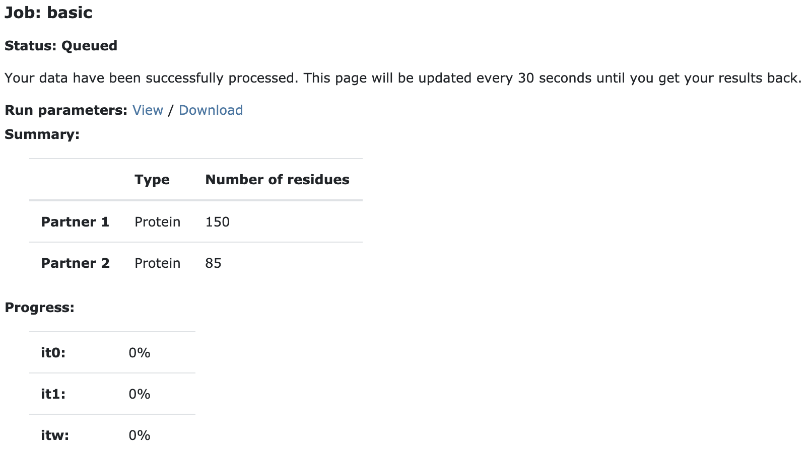
Currently your run should be queued but eventually its status will change to “Running”:

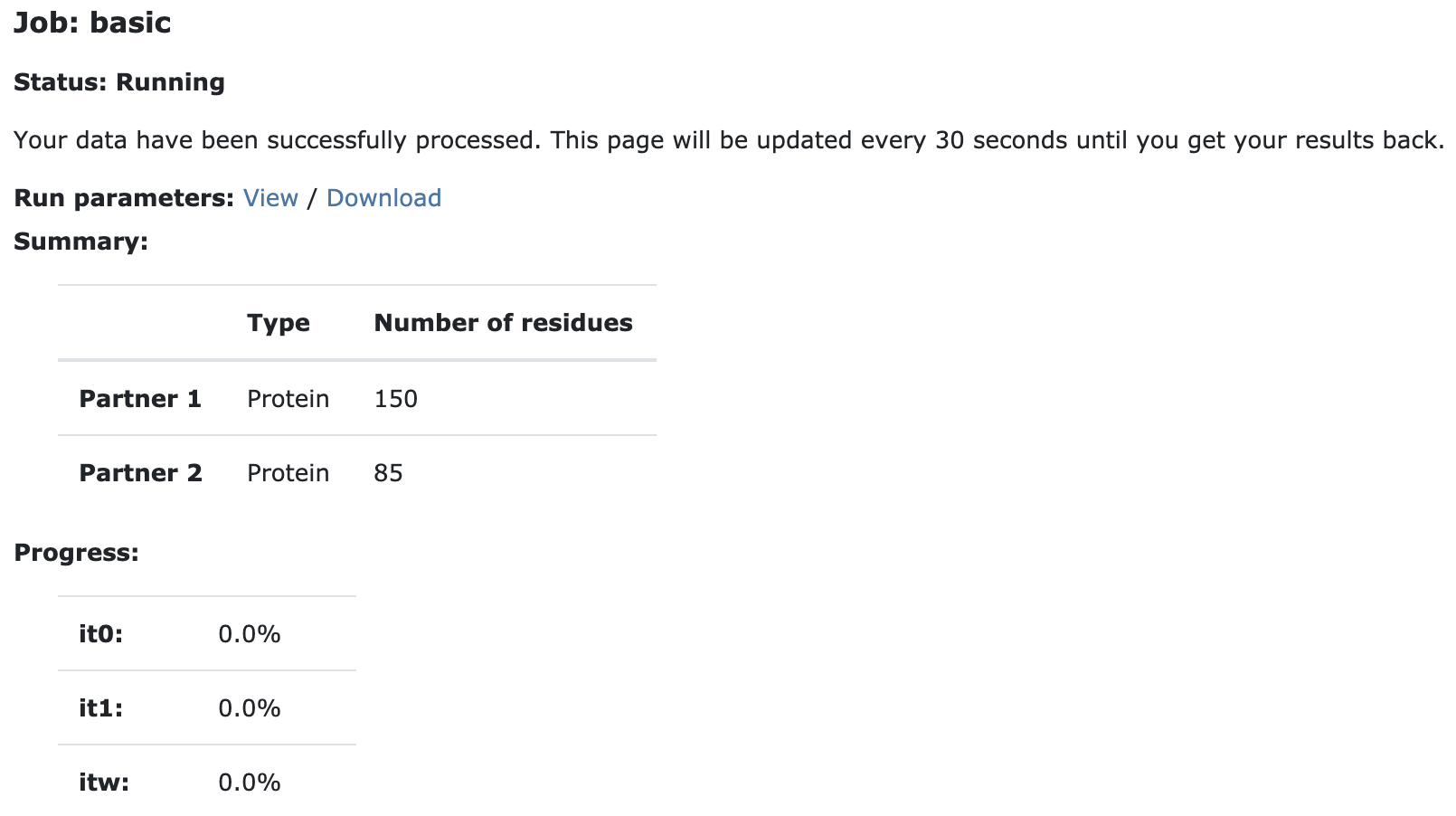
The page will automatically refresh and the results will appear upon completions (which can take between 1/2 hour to several hours depending on the size of your system and the load of the server). You will be notified by email once your job has successfully completed.

Analysing the results

Once your run has completed you will be presented with a result page showing the cluster statistics and some graphical representation of the data (and if registered, you will also be notified by email).

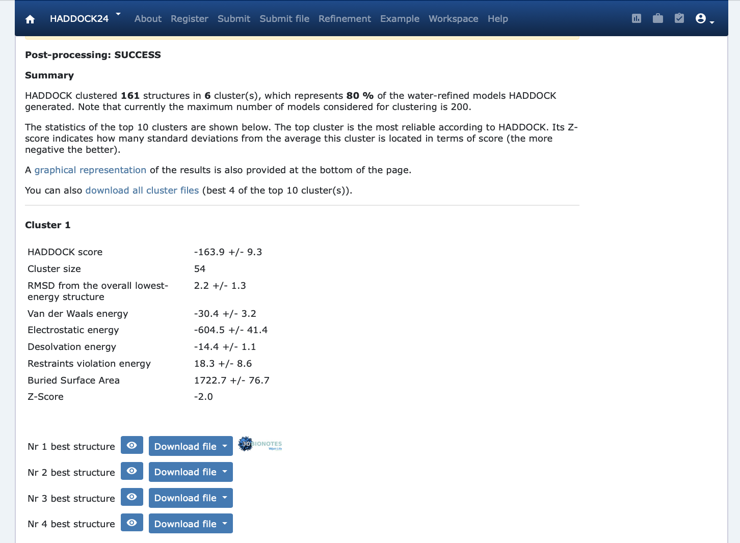
Inspect the result page Q6: How many clusters are generated? Q7: Which is the metric used to sort the clusters? Q8: Look at the cluster names (cluster1, cluster2,…). Can you figure out on which basis is the cluster number assigned (i.e. which displayed metric (various energies, size, …) does it correlate?

Note: The bottom of the page gives you some graphical representations of the results, showing the distribution of the solutions for various measures (HADDOCK score, van der Waals energy, …) as a function of the Fraction of Common Contact and RMSD from the best generated model (the best scoring model). The graphs are interactive and you can turn on and off specific clusters, but also zoom in on specific areas of the plot.

The bottom graphs show you the distribution of scores (Evdw, Eelec and Edesol) for the various clusters.

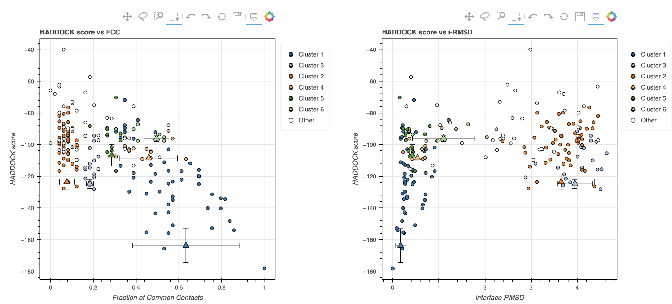
The HADDOCK score is calculated as:

      HADDOCKscore = 1.0 * Evdw + 0.2 * Eelec + 1.0 * Edesol + 0.1 * Eair

where Evdw is the intermolecular van der Waals energy, Eelec the intermolecular electrostatic energy, Edesol represents an empirical desolvation energy term adapted from Fernandez-Recio et al. J. Mol. Biol. 2004, and Eair the AIR energy. The various components of the HADDOCK score are also reported for each cluster on the results web page.

Q9: Consider the cluster scores and their standard deviations. Is the top ranked cluster significantly better than the second one? Q10: The z-scores are calculated based on the HADDOCK scores. What does a z-score of -1.9 mean (Z-scores are handled in the MolMod lecture 7 about structure validation)? You can complement your answer with a graphical and/or mathematical representation.

Ideally, some additional independent experimental information should be available to decide on the best solution. In this case we do have such a piece of information: the phosphate transfer mechanism (see Biological insights below).

Visualisation

The new HADDOCK2.4 server integrates the NGL viewer which allows you to quickly visualize a specific structure. For that click on the “eye” icon next to a structure.

In order to compare the various clusters we will however download the models and inspect them using PyMol.

Download and save to disk the first model of each cluster (use the PDB format)

Then start PyMOL and load each cluster representative:

File menu -> Open -> select cluster1_1.pdb

Repeat this for each cluster. Once all files have been loaded, type in the PyMOL command window:

show cartoon
util.cbc
hide lines

Let’s then superimpose all models on chain A (E2A) of the first cluster:

select cluster1_1 and chain A
align cluster2_1, sele

Repeat the align command for each cluster representative.

This will align all clusters on chain A (E2A), maximizing the differences in the orientation of chain B (HPR).

Q11: Examine the various clusters (the top model from the top 10 clusters). How does the orientation of HPR differ between them? Do attach a picture that supports your answer.

Note: You can turn on and off a cluster by clicking on its name in the right panel of the PyMOL window.

Note: If you aligned correctly the clusters with the commands described above, all clusters shoud be well aligned on E2A, which makes it easier to see differences in the orientation of HPR. Use for example the alpha helix of HpR as a reference to compare orientations.

Let’s now check if the active residues which we defined are actually part of the interface. In the PyMOL command window type:

select e2a_active, (resi 38,40,45,46,69,71,78,80,94,96,141) and chain A
select hpr_active, (resi 15,16,17,20,48,49,51,52,54,56) and chain B
color red, e2a_active
color orange, hpr_active

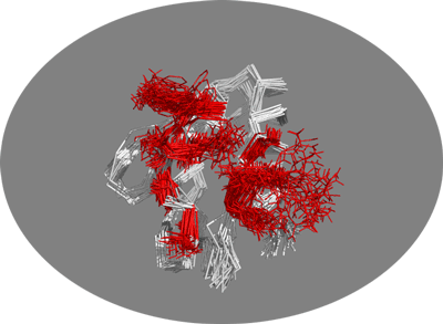
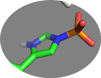
Q12: Are the active residues in the interface? Do attach a picture that supports your answer.

Biological insights

The E2A-HPR complex is involved in phosphate-transfer, in which a phosphate group attached to histidine 90 of E2A (which we named NEP) is transferred to a histidine of HPR. As such, the docking models should make sense according to this information, meaning that two histidines should be in close proximity at the interface. Using PyMOL, check the various cluster representatives (we are assuming here you have performed all PyMOL commands of the previous section):

select histidines, resn HIS+NEP
show spheres, histidines
util.cnc

Note: You can zoom on the phosphorylated histidine using the following PyMOL command:

zoom resn NEP

Zoom back to all visible molecules with

zoom vis

Q13: First of all, has the phosphate group been properly generated? Q14: If so, what is the distance (in angstroms) of the N-P bond? How does it compare with C-C and O-P bonds? TIP: You may calculate them by using the atomic coordinates from the PDB file (open it in a text editor and locate the phosphate atom) or using the “Wizard->Measurement” command in PyMOL (click on the two atoms upon activating the “Measurement“ wizard).

Now inspect each cluster in turn and check if histidine 90 of E2A is in close proximity to another histidine of HPR. To facilitate this analysis, view each cluster in turn (use the right panel to activate/desactivate the various clusters by clicking on their name).

Q15: Based on this analysis, which cluster does satisfy best the biolocal information?

Q16:Is this cluster also the best ranked one? If not what is its rank?

Comparison with the reference structure

As explained in the introduction, the structure of the native complex has been determined by NMR (PDB ID 1GGR) using a combination of intermolecular NOEs and dipolar coupling restraints. We will now compare the docking models with this structure.

If you still have all cluster representative open in PyMOL you can proceed with the sub-sequent analysis, otherwise load again each cluster representative as described above. Then, fetch the reference complex by typing in PyMOL:

fetch 1GGR
show cartoon
color yellow, 1GGR and chain A
color orange, 1GGR and chain B

The number of chain B in this structure is however different from the HPR numbering in the structure we used: It starts at 301 while in our models chain B starts at 1. We can change the residue numbering easily in PyMol with the following command:

alter (chain B and 1GGR), resv -=300

Then superimpose all cluster representatives on the reference structure, using the entire chain A (E2A):

select 1GGR and chain A
align cluster1_1, sele, cycles=0

Repeat the align command for each cluster representative.

Q17: Does any of the cluster representatives ressemble the reference NMR structure (PDB code: 1GGR) NMR structure? If so, what is its cluster rank?

In the blind protein-protein prediction experiment CAPRI (Critical PRediction of Interactions), a measure of the quality of a model is the so-called ligand-RMSD (l-RMSD). It is calculated by fitting on the receptor chain (E2A or chain A in our case) and calculating the RMSD on the backbone of the ligand (HPR or chain B in our case).

Q18: Give and explain the equation to calculate the RMSD.

The RMSD can be calculated in PyMOL with the following command:

rms_cur cluster1_1 and chain B, 1GGR

In CAPRI, the l-RMSD value defines the quality of a model:

acceptable model: l-RMSD<10Å
medium quality model: l-RMSD<5Å
high quality model: l-RMSD<1Å

Q19: What is based on this CAPRI criterion the quality of the best model?

Note: On some machines the pymol rms_cur command can fail due to a bug in the PyMOL software. In this case you can use the following command instead:

align cluster1_1, 1GGR, cycles=0

This will align the two structures based on the all-atom RMSD, different from the ligand-RMSD (l-RMSD) that you can calculate with rms_cur and the above commands.

Congratulations!

You have completed this computer practical. If you have any questions or suggestions, feel free to contact us via email or asking a question through our support center.

Your report

For this practical you should write a report answering all questions above. For your convenience these are again listed here:

Q1: Is there any phosphate group present in the E2A structure? (PDB code: 1F3G). If so, state the residue name and the residue number.

Q2: Do the E2A residues identified by NMR as putative binding form a well-defined patch on the surface? Do they form a contiguous patch? Motivate your answers.

Q3: Do the HpR residues identified by NMR as putative binding form a well-defined patch on the surface? Do they form a contiguous patch? Motivate your answers.

Q4: In contrast to E2A, HPR consists of an ensemble of models. Does this fact provide any advantage for modeling purposes compared to structures solved by X-ray crystallography?

Q5: What is the proper residue name for a phospho-histidine in HADDOCK?

Q6: How many clusters are generated?

Q7: Which is the metric used to sort the clusters?

Q8: Look at the cluster names (cluster1, cluster2,…). Can you figure out on which basis is the cluster number assigned (i.e. which displayed metric (various energies, size, …) does it correlate?

Q9: Consider the cluster scores and their standard deviations. Is the top ranked cluster significantly better than the second one?

Q10: The z-scores are calculated based on the HADDOCK scores. What does a z-score of -1.9 mean (Z-scores are handled in the MolMod lecture 7 about structure validation)? You can complement your answer with a graphical and/or mathematical representation.

Q11: Examine the various clusters (the top model from the top 10 clusters). How does the orientation of HPR differ between them? Do attach a picture that supports your answer.

Q12: Are the active residues in the interface? Do attach a picture that supports your answer.

Q13: First of all, has the phosphate group been properly generated?

Q14: If so, what is the distance (in angstroms) of the N-P bond? How does it compare with C-C and O-P bonds? TIP: You may calculate them by using the atomic coordinates from the PDB file (open it in a text editor and locate the phosphate atom) or using the “Wizard->Measurement” command in PyMOL (click on the two atoms upon activating the “Measurement“ wizard).