

HADDOCKing of the p53 N-terminal peptide to MDM2
General Overview
This tutorial introduces protein-protein docking using the HADDOCK web server. It also introduces the CPORT web server for interface prediction, based on evolutionary conservation and other biophysical properties. By the end of this tutorial, you should know how to setup a HADDOCK run and interpret its results in terms of biological insights.
- A bite of theory
- Predicting the interface of p53 on MDM2
- Preparing the structures for the docking calculation
- Setting up the docking calculation using the HADDOCK web server
- Analyzing the docking calculation results
- Visual inspection of the cluster representatives
- Congratulations!
A bite of theory
Protein-protein interactions mediate most cellular processes in the cell, such as differentiation, proliferation, signal transduction, and cell death. Their structural characterization is however not always trivial, even with the constant developments in X-ray crystallography, nuclear magnetic resonance spectroscopy and cryo electron microscopy. The culprits widely vary, ranging from the native environment of the complexes, which might make them hard to purify or crystallize, to the size of the system being too large for current methodologies to grasp. More importantly, homeostasis often depends on very tightly regulated transient interactions, yet another hindrance to the purification and characterization of these complexes. Nevertheless, three decades of spectacular progress in structural biology have shown that the protein fold space is finite and the rules of the folding game are well defined. This prompted the development of several computational methods aimed at complementing experimental techniques in their quest for a full 3D view of the proteome. A widely used computational method for the prediction of the protein-protein complexes is molecular docking, which aims at generating the structure of such a complex starting from the structures (or models) of its native constituents.
This tutorial will introduce HADDOCK (High Ambiguity Driven DOCKing) as a method to predict the three-dimensional structure of protein-protein complexes in silico using a variety of sources of information to guide the docking process and score the predicted models. HADDOCK is a collection of python scripts derived from ARIA, that harness the power of CNS (Crystallography and NMR System) for structure calculation of molecular complexes. What distinguishes HADDOCK from other docking software is its ability, inherited from CNS, to incorporate experimental data as restraints and use these to guide the docking process alongside traditional energetics and shape complementarity. Moreover, the intimate coupling with CNS endows HADDOCK with the ability to actually produce models of sufficient quality to be archived in the Protein Data Bank.
A central aspect to HADDOCK is the definition of Ambiguous Interaction Restraints (AIRs). These allow the translation of raw data such as NMR chemical shift perturbation or mutagenesis experiments into distance restraints that are incorporated in the energy function used in the calculations. AIRs are defined through a list of residues that fall under two categories: active and passive. Generally, active residues are those of central importance for the interaction, such as residues whose knockouts abolish the interaction or those where the chemical shift perturbation is higher. Throughout the simulation, these active residues are restrained to be part of the interface, if possible, otherwise incurring in a scoring penalty. Passive residues are those that contribute for the interaction, but are deemed of less importance. If such a residue does not belong in the interface there is no scoring penalty. Hence, a careful selection of which residues are active and which are passive is critical for the success of the docking.
The docking protocol of HADDOCK was designed so that the molecules experience varying degrees of flexibility and different chemical environments, and it can be divided in three different stages, each with a defined goal and characteristics:
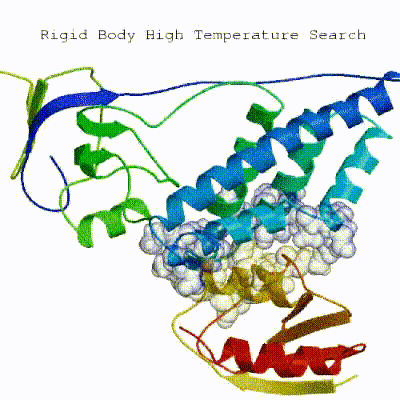
1. Randomization of orientations and rigid-body minimization (it0)
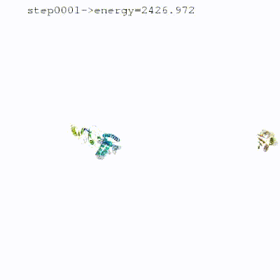
In this initial stage, the interacting partners are treated as rigid bodies, meaning that all geometrical parameters such as bonds lengths, bond angles, and dihedral angles are frozen. The partners are separated in space and rotated randomly about their centres of mass. This is followed by a rigid body energy minimization step, where the partners are allowed to rotate and translate to optimize the interaction. The role of AIRs in this stage is of particular importance. Since they are included in the energy function being minimized, the resulting complexes will be biased towards them. For example, defining a very strict set of AIRs leads to a very narrow sampling of the conformational space, meaning that the generated poses will be very similar. Conversely, very sparse restraints (e.g. the entire surface of a partner) will result in very different solutions, displaying greater variability in the region of binding.
▼ Click here to see animation of rigid-body minimization (it0) ▼
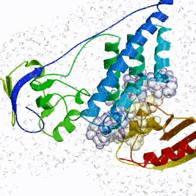
2. Semi-flexible simulated annealing in torsion angle space (it1)
The second stage of the docking protocol introduces flexibility to the interacting partners through a three-step molecular dynamics-based refinement in order to optimize interface packing. It is worth noting that flexibility in torsion angle space means that bond lengths and angles are still frozen. The interacting partners are first kept rigid and only their orientations are optimized. Flexibility is then introduced in the interface, which is automatically defined based on an analysis of intermolecular contacts within a 5Å cut-off. This allows different binding poses coming from it0 to have different flexible regions defined. Residues belonging to this interface region are then allowed to move their side-chains in a second refinement step. Finally, both backbone and side-chains of the flexible interface are granted freedom. The AIRs again play an important role at this stage since they might drive conformational changes.
▼ Click here to see animation of semi-flexible simulated annealing (it1) ▼
3. Refinement in Cartesian space with explicit solvent (water)
Note: This stage was part of the standard HADDOCK protocol up to (and including) v2.2. As of v2.4 it is no longer performed by default but the user still has the option of enabling it. In its place, a short energy minimisation is performed instead. The final stage of the docking protocol immerses the complex in a solvent shell so as to improve the energetics of the interaction. HADDOCK currently supports water (TIP3P model) and DMSO environments. The latter can be used as a membrane mimic. In this short explicit solvent refinement the models are subjected to a short molecular dynamics simulation at 300K, with position restraints on the non-interface heavy atoms. These restraints are later relaxed to allow all side chains to be optimized.
▼ Click here to see animation of refinement in explicit solvent (water) ▼
The performance of this protocol of course depends on the number of models generated at each step. Few models are less probable to capture the correct binding pose, while an exaggerated number will become computationally unreasonable. The standard HADDOCK protocol generates 1000 models in the rigid body minimization stage, and then refines the best 200 – regarding the energy function - in both it1 and water. Note, however, that while 1000 models are generated by default in it0, they are the result of five minimization trials and for each of these the 180º symmetrical solution is also sampled. Effectively, the 1000 models written to disk are thus the results of the sampling of 10.000 docking solutions.
The final models are automatically clustered based on a specific similarity measure – positional interface ligand RMSD (iL-RMSD) – that captures conformational changes about the interface by fitting on the interface of the receptor (the first molecule) and calculating the RMSDs on the interface of the smaller partner. The interface used in this calculation is automatically defined based on an analysis of all contacts made in all models.
Predicting the interface of p53 on MDM2
HADDOCK excels at predicting the structure of the protein complexes given there is some sort of information to guide the docking. In the absence of experimental information, it is possible to use features such as sequence conservation and biophysical characteristics of surface residues to infer putative interfaces on a protein surface. Since the homology modeling module created a list of homologues of mouse MDM2, it is possible to assess which residues are more conserved.
First we need to find sequence homologues again. This time we will be running a BLAST search using Uniprot. We can come back to the entry from the homology modelling part where we looked up mouse MDM2 in Uniprot.
Search for ‘MDM2’ in UniProt and choose the mouse isoform.
A familiar page should appear with all the previously described information. Go directly to the Sequences section. The sequence that you see is a canonical sequence, which means that it is either the most prevalent, the most similar to orthologous sequences in other species or in absence of any information, the longest sequence. On the top-left side of the sequence there is a possibility to run a BLAST (Basic Local Alignment Search Tool) search.
Click on ‘Tools’ next to the canonical sequence and select ‘BLAST’.
Next, a new window will open with the BLAST search. One can enter either a protein or a nucleotide sequence or a UniProt identifier.
This step might take a few moments since our sequence is being compared to the UniProtKB reference proteomes plus SwissProt databases. Once the run is finished, we can see a list of orthologous sequences from different organisms ordered by sequence identity.
Which organism shows the highest sequence similarity to the mouse MDM2? Is it surprising?
To be able to take information about conserved residues and use it in HADDOCK, we need to align selected sequences.
The easiest way to visualize the alignment to identify which positions are more conserved is by generating a sequence logo. For each position in the sequence, the logo identifies the most frequently occurring residues and scales its one-letter code according to a conservation score. We will be using the WebLogo server, in order the generate the sequence logo for the alignment produced by BLAST.
Create the sequence logo by submitting the BLAST alignment file to the WebLogo server.
Since the other sequences might be longer than our query, specify conservancy of which residues you are interested in.
In WebLogo 3, upload your alignment file
Do you see where the mouse MDM2 sequence is located on the alignment? Try to select residues 146-231 in logo range.
Which regions of the sequence are highly conserved? And which are less conserved?
Visualize the homology model of mouse MDM2 in PyMOL.
Predicting interface residues
Besides sequence conservation, other features can be used to predict possible interfaces on protein structures. For example, certain residues tend to be overrepresented at protein-protein interfaces. This information, combined with evolutionary conservation and with a surface clustering algorithm that finds groups of surface residues meeting both the previous criteria results in reasonably accurate predictions. This is the basis of the WHISCY server. A more advanced predictor, the CPORT web server, judiciously combines (up to) 6 different predictors to provide a consensus prediction that is more robust and more reliable than any of the individual predictors alone.
Many tools in science are developed by dedicated PhD students and postdocs. Unfortunately, over time, some of these tools may become unavailable as maintaining and supporting them requires significant time and effort. In such cases, it may be necessary to use alternative tools.
Obtain known interfaces of homologous proteins
Another way to obtain information about possible interface residues is by analysing known interfaces found in homologous proteins. This can easily be performed by ARCTIC-3D, a tool dedicated to an automatic retrieval and clustering of interfaces in complexes from 3D structural information. As structural information of the human MDM2 interacting with other partners is available, ARCTIC-3D will extract interacting residues and cluster them into binding surfaces. Not all residues of a binding surface are relevant, as some amino acids may be rarely present among the interfaces that define that patch. Wisely define a probability threshold and note down the residue indices, as you will need them to define active residues in HADDOCK.
By selecting the ‘Cluster partners by protein function’ option the software will look into the function of the protein partners that interact with each binding surface.
Download the outputs of ARCTIC-3D. ARCTIC-3D will provide a structure of the human MDM2, and add the residue contact probability in the b-factor column, enabling to easily visualise it on PyMOL.
Because the current residue indices match the human canonical sequence, you will have to run a structural alignment of your mouse MDM2 model onto this structure and define the residue mapping by hand.
For this, you need to load your mouse MDM2 model on the same PyMOL session and then perform a structural alignment on the human one. The align function, already implemented in PyMOL, is easy to use and well suited for this task.
align mouse_model, human_structure
What is the list of residues indices that you selected?
Preparing the structures for the docking calculation
In order to perform a docking calculation with HADDOCK, the initial structures of both MDM2 and p53
must fulfill a few requirements. First, the PDB files must have an END statement as a last line.
The files can also not contain atoms with multiple occupancies. It is however possible to submit an
ensemble of structures, which is useful for the representatives of p53 extracted from the molecular
dynamics simulation. When submitting such an ensemble, all members must contain exactly the same atoms.
Luckily, both the files produced by SWISS-MODEL and by GROMACS respect the END statement and multiple occupancy
requirement, so no action is necessary here.
The structures of the p53 peptide originating from the molecular dynamics simulation can be
submitted as a single ensemble to HADDOCK. The pdb_mkensemble utility of the pdb-tools set
provides a quick way of building such an ensemble structure from isolated PDB files. It also adds
the proper END statement to the PDB file. Finally, it has a built-in check for the integrity of
the ensemble, i.e. that all members have exactly the same atomic constitution.
Concatenate different representatives of the MD simulation of the p53 peptide into an ensemble structure. pdb_mkensemble p53_cluster_1.pdb p53_cluster_2.pdb p53_cluster_3.pdb > p53_ensemble.pdb
Setting up the docking calculation using the HADDOCK web server
Registration / Login
To get an HADDOCK account go to https://wenmr.science.uu.nl/haddock2.4/ and click on Register.
Having prepared the initial structures and constructed a list of putative interface residues, it is time to submit the docking calculation using the HADDOCK 2.4 web server.
Here, you can useful information for example a link to the new HADDOCK best practice guide, which comprises settings for different docking scenarios. Under the Server Information section in the web page, you can find a link to the default settings of the webserver, which are important to understand how restraints for example are handled, as well as a list of supported modified amino acids and co-factors and the current HADDOCK version.
To start the job submission, click on Submit a new job.
Submission and validation of structures
For this we will make use of the HADDOCK 2.4 submission interface of the HADDOCK web server.
-
Step 1: Define a name for your docking run in the field
Job name, e.g. MDM2-p53. -
Step 2: Select the number of molecules to dock, in this case the default 2.
-
Step 3: Input the first protein PDB file. For this unfold the
Molecule 1 - inputif it isn’t already unfolded.
Which chain to be used? -> All (for this particular case) PDB structure to submit -> Browse and select modelx.pdb (the homology model you prepared before)
Note: Leave all other options to their default values.
- Step 4: Input the second protein PDB file. This is the ensemble of three peptide conformations. For this unfold the
Molecule 2 - inputif it isn’t already unfolded.
Which chain to be used? -> All (for this particular case) PDB structure to submit -> Browse and select p53_ensemble.pdb (the PDB file containing the ensemble of peptide models you prepared before)
Since our homology model and peptide do not correspond to the full sequence it is better to have uncharged termini.
- Step 5: Click on the
Nextbutton at the bottom left of the interface. This will upload the structures to the HADDOCK webserver where they will be processed and validated (checked for formatting errors). The server makes use of Molprobity to check side-chain conformations, eventually swap them (e.g. for asparagines) and define the protonation state of histidine residues.
Definition of restraints
If everything went well, the interface window should have updated itself and it should now show the list of residues for molecules 1 and 2. We will be making use of the text boxes below the residue sequence of every molecule to specify the list of active residues to be used for the docking run. The definition of restraints does require some thoughts. Active residues in HADDOCK are those that are required to be at the interface. Passive residues, on the other hand, are those that might be at the interface. Ambiguous Interaction Restraints, or AIRs, are created between each active residue of a partner and the combination of active and passive residues of the other partner. An active residue which is not at the interface will cause an energy penalty while this is not the case for passive residues. For the docking of MDM2 and p53, define active residues on MDM2 based on ARCTIC-3D output. As there is no information about interacting residues for the peptide, define entire p53 as passive. This follows the recipe published in our Structure 2013 paper. In that way the active residues of the protein will attract the peptide, while peptide residues do not have all to make contacts per se.
- Step 6: Specify the active residues for the first molecule. For this unfold the
Molecule 1 - parametersif it isn’t already unfolded. In this stage we will make use of the active residues returned by CPORT for MDM2
Active residues (directly involved in the interaction) -> Input here the list of active residues returned by ARCTIC-3D for MDM2 Automatically define passive residues around the active residues -> uncheck (passive should only be defined if active residues are defined for the second molecule)
- Step 7: Specify the active residues for the second molecule. For this unfold the
Molecule 2 - parametersif it isn’t already unfolded.
Active residues (directly involved in the interaction) -> Leave blank (no active for the peptide in this case) Automatically define passive residues around the active residues -> uncheck (checked by default) Passive residues (surrounding surface residues) -> Enter here all residues of the peptide as a comma-separated list
Note: Notice that instead of typing all residues manually, you can select them from the sequence above. Secondary structure is represented in different colors.
Definition of fully flexible segments
- Step 8: Since peptides are highly flexible we will give more flexibility to the peptide to allow for larger conformational changes. For this unfold the
Fully flexible segments tabfor molecule 2 and enter:
Fully flexible segments -> Enter here all residues of the peptide as a comma-separated list
Here you can also simply select the entire peptide sequence again. This will cause HADDOCK to consider the peptide residues as fully flexible during all stages of the simulated annealing refinement stage and therefore increase sampling.
Increased sampling
If we don’t fully trust our information about binding, it is safer to increase sampling to consider more solutions.
- Step 9: This can be done in one simple step by choosing the bioinformatics predictions settings described here.
Optimize run for bioinformatics predictions -> check
- Step 10: Click on the
Nextbutton on the bottom of the page.
Checking the bioinformatic prediction setting changes automatically sampling to these parameters:
Number of structures for rigid body docking -> 10000 Number of structures for semi-flexible refinement -> 400 Number of structures for the final refinement -> 400 Number of trials for rigid body minimisation -> 1 Number of structures to analyze -> 400
The use of an ensemble of structures translates into a worse sampling per conformation at the rigid-body stage.
Each starting conformation will be sampled a limited number of times as defined by the total number of models sampled
at the rigid-body docking stage divided by the number of models in the ensemble. With the default values of 1000 rigid-body models,
an ensemble of 10 starting conformations translates to 100 models generated per member of the ensemble.
This reduction in sampling per model might deteriorate the accuracy of the docking calculations,
particularly if the restraints are fuzzy, as is the case when using bioinformatics predictions.
For this reason it is recommended to increase the number of structures generated at
the various stages of the docking protocol. As a rule of thumb, 1000 rigid-body models per member
of the ensemble is a good number. The number of models selected to it1 and water can simply be
doubled. The computational cost of these refinement stages does not allow a proportional increase.
These numbers can be edited one by one in the Sampling parameters tab, but are done automatically when checking the Bioinformatics predictions setting.
Note: Because of the decreased sampling per model in the case of an ensemble of starting structures, it is recommended to limit the number of conformations in the starting ensembles. This is even more important if ensembles of conformations are used for each molecule to dock. For example, 10 models per molecule will generate 100 combinations in the case of two molecule docking. With a sampling of 10000 at the rigid body docking stage, each combination will only be sampled 100 times. Note that the server limits the number of it0 models to a maximum of 10000.
Clustering parameters
- Step 11:
For this unfold the
Parameters for clustering menu.
HADDOCK offers two different clustering algorithms. Refer to the online manual for more details. For peptide and small molecules we recommend the use of RMSD clustering. The clustering algorithm must also be adjusted to accommodate the small size of the peptide. The default cutoff of \(7.5Å\) (interface-ligand RMSD) was optimized for protein-protein docking and is very likely too large in the case of protein-peptide complexes. Clustering with this value would very likely generate very large and diverse clusters. We should therefore reduce the clustering cutoff:
Clustering method (RMSD or Fraction of Common Contacts (FCC)) -> Select RMSD RMSD Cutoff for clustering (Recommended: 7.5A for RMSD, 0.75 for FCC) -> 5.0
Automatic restraining of secondary structure elements
- Step 12: For this unfold the
Dihedral and hydrogen bonds restraints menu.
HADDOCK offers an option to automatically define dihedral angle restraints based on the input structure. This can be applied either to the entire sequence, or only to alpha helical segments or to alpha and beta segments. These are automatically detected based on the measured dihedral angles. For flexible peptides, since we are treating them as fully flexible, it is recommended to turn on this option.
Automatically define backbone dihedral restraints from structure? -> Select Only for alpha helix
Advanced sampling parameters
- Step 13: Adjust the number of flexible refinement steps to increase the sampling of peptide conformations in
Advanced sampling parametersmenu.
Double the number of steps for all four stages of the semi-flexible refinement:
number of MD steps for rigid body high temperature TAD -> 1000 number of MD steps during first rigid body cooling stage -> 1000 number of MD steps during second cooling stage with flexible side-chains at interface -> 2000 number of MD steps during third cooling stage with fully flexible interface –> 2000
Job submission
This interface allows us to modify many parameters that control the behavior of HADDOCK but in our case the default values are all appropriate. It also allows us to download the input structures of the docking run (in the form of a .tgz archive) and a parameter file which contains all the settings and input structures for our run (in .json format). We strongly recommend to download this file as it will allow you to repeat the run afterwards by uploading into the file upload interface of the HADDOCK web server. It can serve as input reference for the run and added to the supplementary material of your publications. This file can also be manually edited.
- Step 14: Click on the
Submitbutton at the bottom left of the interface.
Upon submission you will be presented with a web page which also contains a link to the previously mentioned haddockparameter file as well as some information about the status of the run.
The second link points to the results page of the simulation. Since a regular docking simulation lasts, on average, a couple of
hours, this page displays its current status while not complete as PROCESSING, QUEUED, or RUNNING. In
case a critical error prevents the simulation from continuing, whether because of problems with the
input data, or problems during the simulation itself, the webpage displays an ERROR message. Most
of these status changes are accompanied by an e-mail that is sent to the address linked to the user
account. In case of errors, this e-mail also offers additional details on the cause(s). For
students, since all accounts are pre-configured, the email notification is turned off.
Analyzing the docking calculation results
After the simulation is complete, the results page is generated and a notification email sent to the user. This results page includes an overview of the top ten clusters, ranked by average HADDOCK score of their four best structures, including statistics of energetic terms and other structural measures for each cluster. This allows a quick assessment of the quality of the generated models. Furthermore, at the bottom of the page, several plots of different quality-control measures of the models also give the opportunity of checking the quality of the docking simulation at a glance.
Visual inspection of the cluster representatives
Any molecular simulation, docking included, lacks the accuracy to produce one single good model.
However, with sufficient attempts, reasonable models are likely to populate the results. HADDOCK in
particular, given its data-driven character, produces much higher quality models if the quality
of the data is good enough. At the end of the simulation, all the models are clustered so as to
filter out the isolated structures that resemble few others in the pool of models. The models are
then analyzed on a cluster basis and the best models of the best clusters are considered the best
representative models of the simulation. Nevertheless, a careful visual inspection is of paramount
importance and should always be the first step of any simulation analysis. To better visualize the
differences between each cluster, superimpose all models onto the backbone of the largest partner,
in this case the MDM2 molecule. For this we have to select a reference model, which we
arbitrarily define as that of cluster1_1.
If your simulation produced several clusters, download the top-ranking model of each cluster and open them in Pymol. If there is only one cluster, open the top four best models of that cluster. select refe, cluster1_1 and chain A align cluster2_1, refe align cluster3_1, refe …
Do the models have any unreasonable feature, such as atomic clashes or unphysical interactions? Based on the best scoring clusters, can you advance a putative binding interface for p53 on MDM2? Can you identify key residues that might be “hotspots” of this interaction?
The best way to validate your docking is to compare your solution to an experimental structure. Luckily for us, there is a human MDM2 bound to the transactivation domain of p53 under PDB code: 1YCR. One can download this complex or simply fetch it with Pymol.
Congratulations!
The docking calculation of MDM2 and the p53 N-terminal transactivation peptide was the culmination of a three-stage computational exercise that involved the three major methods in the repertoire of a Computational Structural Biologist. As you have seen, in modeling, there are rarely any certainties and you must always operate with extreme care and a constant sense of (self-)criticism. Nevertheless, you started with only two sequences and have now three-dimensional models of interactions that can be put to the test in the lab. Who knows? Maybe one of your models is actually correct and it will help researchers to spare the life of a few of our mice friends! 🐁
Thank you for following this tutorial. We welcome any feedback to improve it. For the students following the course Molecular Modeling and Simulation, please feel free to voice any criticism and/or suggestions to the instructors. You won’t be negatively judged for it :) Others may send comments to the email on the right side of the page, under the head of Captain HADDOCK!